
What Is VLOOKUP From Another Google Sheet?
The VLOOKUP function in Google Sheets retrieves the required data from the dataset based on the search_key within the same worksheet of the workbook.
VLOOKUP From Another Google Sheet helps us work on scenarios where we may have to retrieve the information from a different Google Sheet in the same workbook or a different workbook.
Use this VLOOKUP From Another Google Sheet Template to follow along with the examples in this article.
Download Excel TemplateFor example, the first table consists the items, their categories and quantities in the “Definition” worksheet. We will find the category for the item cited, here, Oranges, in the “Definition Result” worksheet with the data table from the first worksheet.

Select cell B16, enter the formula =VLOOKUP(A16,Definition!A11:C17,2,0) and press “Enter”.
The output is shown above as Fruit.

The output is returned as Fruit. The formula retrieves the value for the “Definition Result” worksheet, from the dataset in the “Definition” worksheet.
Key Takeaways
- The VLOOKUP function from Another Google Sheet can fetch the data from different Google Sheets within the same workbook or an entirely different workbook.
- We can fetch the data from different Google Sheets of the same workbook by manually entering the range details for the range argument or by selecting the dataset range. Regardless of how we enter the range, we will get the Google Sheet name along with the range.
- When we apply the VLOOKUP function from different Google Sheets, we can also create named ranges.
- To apply the VLOOKUP from different workbooks, we must use the IMPORTRANGE function.
How To Use VLOOKUP From Another Google Sheet (Same Workbook) ?
We can use the VLOOKUP From Another Sheet from the Same Workbook as any other VLOOKUP formula. However, follow the guidelines given below.
- The dataset will be in a worksheet and the formula applied result cell will be in another worksheet, but, both worksheets will be in the same workbook.
- We need to switch to the different Sheets to select the range for the VLOOKUP function.
Examples
Let us consider a couple of examples to use the VLOOKUP From Another Google Sheet from the Same Workbook.
Example #1
Consider the following data in the “Employee Master” Google Sheet, we have the employee list and all the other necessary information.

We have another worksheet named the “Resigned Employees” in the same workbook, with the following information.

In this Google Sheet, we have the list of employees who have resigned in the current month and need to identify the “City” they belong to from the first Google Sheet, “Employee Master”.
The steps to use the VLOOKUP function are,
Step 1: In the “Resigned Employees” sheet, select cell C2 and enter the formula =VLOOKUP(A2,

Step 2: We see in the image above it is asking for the range. Now, we must enter the cell range from the “Employee Master” sheet. Then, the formula becomes =VLOOKUP(A2,’Employees Master’!A1:F12, as shown below.

Step 3: Since we must apply the same formula to different employees, make the range selection absolute, by pressing the F4 key once and the dollar symbols get inserted, as shown.
[Note: In some systems, the F4 key works, but, in some we might have to use the “Fn+F4” keys.]

Step 4: Do not switch to the “Resigned Employees” Sheet. Stay in the range selection sheet, and enter the index as 4 to get the city information from the 4th column of the range selection and enter the [is_sorted] as FALSE or 0 to get the exact match, as shown below.

Step 5: Finally, close the brackets and press “Enter”. The complete formula is =VLOOKUP(A2,’Employees Master’!$A$1:$F$12,4,0).
Immediately, we are back to the “Resigned Employees” sheet with the VLOOKUP retrieving the city name for the first resigned employee “Los Angeles”, as shown below.

Step 6: Drag the formula from cell C2 to C5 using the fill handle to get the results, as shown below.

Example #2 – VLOOKUP From Another Google Sheet with Named Ranges
We have the data given below from the “Ex 2 – Named Range” worksheet, that consists employee names, their designations and joining dates. Let us find the joining date of the employee, here, Tabita, by giving a defined name to the table array or the cell range.

We have another worksheet named the “Ex 2 – Result Sheet” in the same workbook, with the following information.

The steps to find the required data using VLOOKUP and the name range are as follows:
Step 1: Let us first create the named range.
First, in the “Ex 2 – Named Range” worksheet, select the “Data” tab à click the “Named ranges” option, as shown below.

Next, the “Named ranges” window appears on the right side. Here, click the “Add a range” option, as shown below.

The following window appears below.

Finally, enter the name “Emp_Data” in the first field, enter or select the cell range, ‘Ex 2 – Named Range’!A11:C17 in the second field, click “OK” and then, click “Done”, as shown below.

We can see the named range, i.e., Emp_Data, created as shown below.

Step 2: To find the required employee’s date of joining, select cell B16 in the “Ex 2 – Result sheet”, enter the formula =vlookup(A16,emp . Immediately we see the created named range, as shown below.

Step 3: Select the named range and complete the formula. The complete formula is =VLOOKUP(A10,Emp_Data,3,0).

Step 4: Press “Enter” to get Tabitha’s joining date, as shown below.

- We created the source dataset as a named range in one worksheet, Emp_Data, which enables the function to search for the lookup value, Tabitha, in the first column of the source data.
- The argument index value is 3. It implies that the function must return the required value from the third column, column C, counted from the first column in the specified table array.
- So, once the function finds its first occurrence in the first column, cell A14, it returns the data in the same row of the column specified by col_index_num, cell C14 value, 4/10/2024 in the result worksheet, i.e., another worksheet, but the same workbook.
How To Use VLOKUP From Another Google Sheet (Different Workbook)?
The VLOOKUP From Another Sheet from Different Workbook works as same as any other VLOOKUP formula. The exception is that, here, the dataset will be in a worksheet and the formula applied result cell will be in another worksheet. But, both worksheets will each be in different workbooks.
Example #1 – VLOOKUP from Different Workbook
In Excel, we can just select the data range from a different workbook, just like how we did for a different worksheet from the same workbook. In Google Sheets, it is not possible. Therefore, we use the IMPORTRANGE function to perform the same.
The IMPORTRANGE function has the following syntax,

Where, the spreadsheet_url is the data workbook link where the data range is present and the range_string is the worksheet name of the data workbook and the dataset range. It will be entered as “worksheet name!dataset range”. We will see the usage in the following example.
We have created two workbooks, namely,
- VLOOKUP from Another Google Sheets with employee details such as ID, name, salary and department in the worksheet, named as Data-Sheet.
- Result Workbook with the Emp ID and the salary details in the worksheet, named as Result-Sheet to retrieve from the other workbook

The steps to retrieve data from the VLOOKUP from Another Google Sheets to the Result Workbook are as follows:
Step 1: In the Result Workbook, select cell B2 and enter the formula =VLOOKUP(A2,

Step 2: Now, go to the main data workbook, i.e., the VLOOKUP from Another Google Sheets workbook. And copy the URL as shown below.

Step 3: Now, come back to the result workbook where we are entering the formula. There, continue typing the IMPORTRANGE function first. Then, open the brackets and paste the URL which we copied earlier, in double-quotes, as shown below. =VLOOKUP(A2,IMPORTRANGE(https://docs.google.com/spreadsheets/d/1o4lq41Cs1XsVeprSqU13hbd06BaLZmlRtdE74rDJpao/edit#gid=1537577952

Step 4: Next, enter the range_string, in our case it is “Date-Sheet!A1:D21”, i.e., the worksheet name in the data workbook along with the dataset range. Then close the brackets for the IMPORTRANGE function, as shown below.

Step 5: Finally, complete the VLOOKUP formula. Therefore, the complete formula will be, =VLOOKUP(A2,IMPORTRANGE(“https://docs.google.com/spreadsheets/d/1o4lq41Cs1XsVeprSqU13hbd06BaLZmlRtdE74rDJpao/edit#gid=1537577952″,”Data-Sheet!A1:D21”),3,0)

Step 6: Press “Enter” to get the result, as shown below.

Step 7: Drag the formula from cell B2 to B21 using the fill handle to get the results, as shown below.

Therefore, we can retrieve data from one workbook to another workbook using the VLOOKUP and the IMPORTRANGE functions.
Important Things To Note
- The named range makes the selected data range an absolute reference. So there is no need to use the F4 key.
- Whenever we select the range from different workbooks, the range selection becomes an absolute reference by default.
- If we use the named range for the range and it gets deleted, then we will get the #NAME? error.
- When we apply the VLOOKUP from another workbook do not delete the source workbook. Then, we will lose the data in the formula sheet.
Frequently Asked Questions (FAQs)
The VLOOKUP function in Google Sheets is found as follows:
Select the “Insert” tab – click the “Function” option right arrow – click the “Lookup” option right arrow – select the “VLOOKUP” function, as shown below.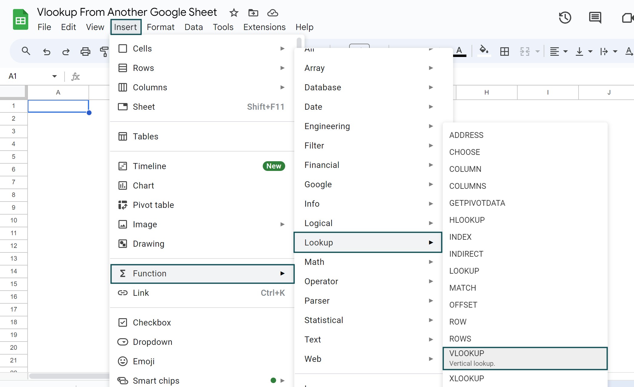
The IMPORTRANGE function in Google Sheets is found as follows:
Select the “Insert” tab – click the “Function” option right arrow – click the “Web” option right arrow – select the “IMPORTRANGE” function, as shown below.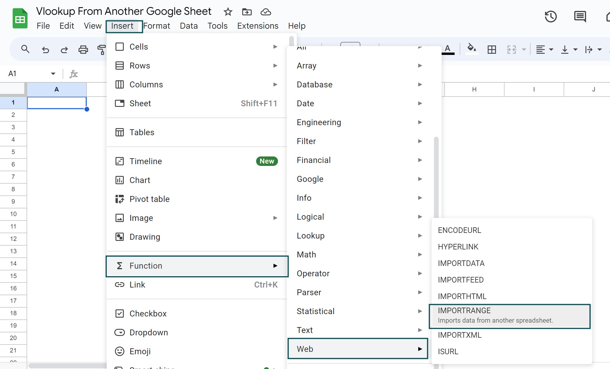
A few reasons the VLOOKUP from Another Google Sheets may not work are,
• If we are getting the #N/A error, then the search_key is not available in the range that we have specified. Even if the parenthesis is not closed or missed, we get the same error with a note “formula phase error”.
• If we get the #REF error because after the VLOOKUP is applied, the range must have been deleted or the index provided is not within the range of the datasets range.
Use this VLOOKUP From Another Google Sheet Template to follow along with the examples in this article.
Download Excel TemplateRecommended Articles
Continue with these related resources when you want the next practical step in this topic.
- LOOKUP in Google Sheets
- HLOOKUP In Google Sheets
- VLOOKUP Table Array In Google Sheets
- VLOOKUP True In Google Sheets
- INDEX MATCH Function In Google Sheets
Explore the full Google Sheets Lookup Functions guide or browse Google Sheets Resources.