What Is CHISQ.DIST.RT Excel Function?
The CHISQ.DIST.RT Excel function is a statistical function used to calculate the right-tailed probability of the chi-square distribution. CHISQ.DIST.RT calculates the right-tailed probability of a chi-square distribution, allowing us to compare observed and expected values. In financial analysis, this function can be used to analyze the relationship between variables such as revenues and customer location. A small value indicates a little relationship, while a larger value suggests a stronger relationship
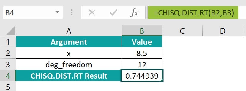
In the following example, let us look at the CHISQ.DIST.RT Excel function and how it works. Here, we have two values: x, the value at which the chi-squared distribution is calculated, and deg_freedom, the degrees of freedom. Apply the formula below in cell B4 to get the result.
= CHISQ.DIST.RT(B2,B3)

Table of contents
Key Takeaways
- The CHISQ.DIST.RT Excel function is used in statistics to calculate the right-tailed probability of the chi-square distribution. It helps compare observed and expected values and can be useful in financial analysis to determine the relationship between variables like revenues and customer location.
- The syntax of CHISQ.DIST.RT Excel function in Excel; =CHISQ.DIST.RT(x,deg_freedom).
- The CHISQ.DIST.RT Excel function is particularly useful in hypothesis testing, where researchers compare observed data with expected data to determine if there is a significant relationship between variables.
- It is used to calculate the probability of finding a value to the right of a specific point in a chi-squared distribution.
Syntax

- x – (Mandatory) This is the value that should be used to calculate the chi-square distribution, and it must be equal to or greater than zero.
- Deg_freedom – (Mandatory) This refers to the number of possible ways a system can move or change. It must be a whole number between 1 and .
How To Use CHISQ.DIST.RT Function in Excel?
To effectively utilize the CHISQ.DIST.RT function in Excel, follow these steps.
#1 – Access from the Excel ribbon
- To display the result in a specific cell, choose an empty cell and click on the Formulas tab.

- To access additional features, go to the menu and choose More Functions.

- Select the Statistical option from the drop-down list and then choose CHISQ.DIST.RT.

- Enter the values of x and degrees of freedom fields in the Function Arguments window. Click OK to continue.

#2 – Enter the worksheet manually
Step 1: To designate an empty cell for the output, simply enter “= CHISQ.DIST.RT()” in the desired cell. Alternatively, you can type “=C” and then double-click on the “CHISQ.DIST.RT” function from the list of suggestions provided by Excel.

Step 2: To achieve the desired result, enter the value and press the Enter key.

Examples
Example #1 – Goodness Of Fit Test
The CHISQ.DIST.RT works by applying a right-tailed probability of the chi-square distribution. In this example, we will compare the actual proportions of coins in some bags to the expected proportions using a goodness of fit test.
The Goodness of fit test using the CHISQ.DIST.RT Excel function is a statistical method used to determine whether there is a significant difference between an observed frequency distribution and the expected frequency distribution. This test is commonly used in research, quality control, and various other fields to assess the validity of a hypothesis.
Step 1: In column D we calculate the value of .
The formula for the calculation is (Observed-Expected^2)/Expected.

Step 2: Using the SUM function, input the formula =SUM(D2:D5) in cell B7 to calculate the Chi-Square value.

Step 3: Input the expression ‘=4-1′ in cell B8 to get the degree of freedom, a value one less than the number of observed values.

Step 4: The value of x and deg of freedom is calculated above. Now, we give the reference values to calculate the right-tailed probability of the Chi-Square distribution for the given test statistic.
=CHISQ.DIST.RT(B7,B8)
Step 5: The outcome is showcased in cell B9.

By passing the required arguments, the formula determines the right-tailed probability for four bags for the Goodness of fit test.
Example #2
Below is data in a table. The value at which we want to evaluate the distribution is 40, and the degree of freedom is 10. Let us calculate its right-tailed probability.

Step 1: To use the CHISQ.DIST.RT formula, select cell B4 and enter the formula as shown.
=CHISQ.DIST.RT(B2,B3)

Step 2: Press enter to see the result in cell B4.

The right-tailed probability of the chi-square in Excel is a statistical measure that indicates the likelihood of obtaining a particular chi-square value or a more extreme value based on a given degree of freedom. In inferential statistics, this probability value is critical for determining the significance of relationships between categorical variables in a contingency table analysis.
Example #3
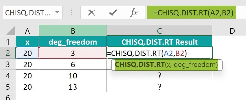
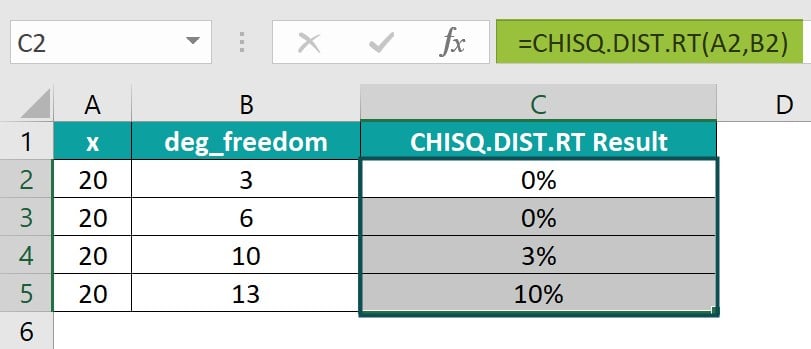
We have an example of having a set of x values and degree of freedom values. We will be calculating probability results in percentages using the CHISQ.DIST.RT Excel function.

Let’s start the calculation by entering the values as prescribed below;
Step 1: Insert the formula to calculate the probability in cell C2. The complete formula is =CHISQ.DIST.RT(A2,B2)

Step 2: The right-tailed probability value is attained in cell C2. Drag the Autofill handle up to C5 to get the results for the other values.

Important Things To Note
- The #VALUE! error occurs when non-numeric arguments are provided. CHISQ.DIST.RT only accepts numeric datasets and returns numeric data.
- The #NUM! error occurs when the value of x is negative or when the deg_freedom argument is less than 1 or greater than .
- If the degrees of freedom argument is not a whole number, it will be rounded down to the nearest whole number.
- It is imperative to remember that this function calculates the right-tailed chi-squared probability distribution. It means that it provides the probability that a value of the chi-squared statistic is greater than a specified value.
- It is important to note that the chi-squared statistic measures how well an observed set of values matches an expected set of values, making it valuable in hypothesis testing and statistical analysis.
- Using the function, it is crucial to input the correct degrees of freedom and cumulative probability to obtain accurate results.

Frequently Asked Questions (FAQs)
While using the CHISQ.DIST.RT Excel function, it is essential for professionals to pay attention to potential errors that may arise during computation.
One common mistake that users may encounter is inputting incorrect values for the degrees of freedom or the probability parameter.
Another error to watch out for is entering a negative value, as this will result in a #NUM! Error being displayed.
Let us look at an example to understand the errors that can pop up when using the CHISQ.DIST.RT Excel function. The table has a list of parameters to be used in the formula.
Type the below formula in cells B6 & C6:
= CHISQ.DIST.RT(B2,B3) in cell B4
= CHISQ.DIST.RT(C2,C3) in cell C4
We get a #VALUE error because the number_sample value is non-numeric.
We get a #NUM! Error because the x value is negative.
The CHISQ.DIST.RT function in Excel differs from other Chi-square distribution functions such as CHIDIST, CHIINV, and CHITEST in its ability to calculate the right-tailed probability of a Chi-square distribution.
• The CHIDIST function returns the probability that a variable is less than or equal to a specified value given a Chi-square distribution.
• The CHIINV function returns the inverse of this probability.
• The CHITEST function performs hypothesis testing by comparing observed and expected frequencies within contingency tables.
In contrast, the CHISQ.DIST.RT function solely focuses on calculating the probability that a Chi-square statistic falls to the right of a specified value, making it particularly useful for determining statistical significance in one-tailed tests where data is skewed in one direction.
The limitation to using the CHISQ.DIST.RT functions are;
• The CHISQ.DIST.RT Excel function assumes a one-tailed hypothesis test, meaning it only calculates the probability of observing a chi-square value greater than the specified value.
• The function requires inputting degree of freedom, which limits its use to problems where this parameter is known.
• This function relies on approximate calculations and may not be as accurate as more advanced statistical software packages for complex distributions or large datasets.
Download Template
This article must help us understand the CHISQ.DIST.RT Excel Function’s formula and examples. You can download the template here to use it instantly.
Recommended Articles
Guide to CHISQ.DIST.RT Excel Function. Here we explain how to use CHISQ.DIST.RT function with examples & downloadable excel template. You can learn more from the following articles –


Leave a Reply