What Is Count Cells By Color In Excel?
The techniques to count cells by color in Excel enable one to calculate the total number of colored cells in a chosen range. We can also filter and count the cells highlighted in a specific color in the given range.
Users can apply the options to count cells by color in Excel while analyzing sales reports and financial statements containing categories of data in different colors.
📥Download the ready-to-use Excel template to practice this tutorial yourself.
Count Cells By Color In ExcelFor example, the table below lists students and their teams. And each team appears highlighted in a unique color.

The requirement is to count the column B cells highlighted in each color and display the outcome in cell B13.
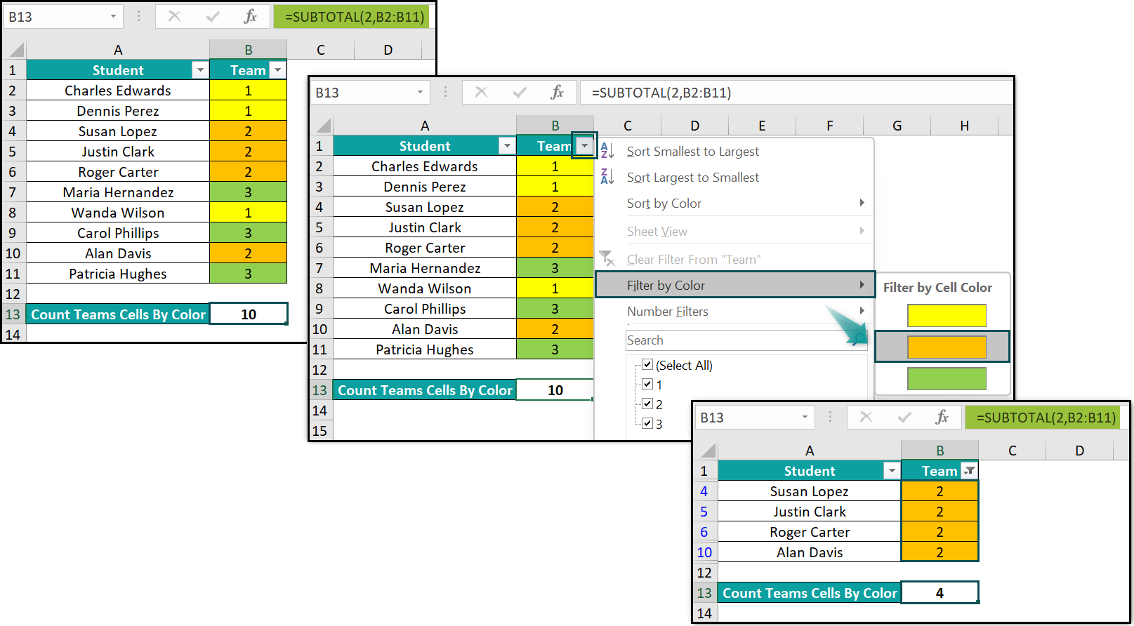
Then, we can apply the count cells by color in Excel formula based on the Excel SUBTOTAL Function in the target cell and the Filter option in the Data tab to achieve the desired output.
In the above example, the first argument in the SUBTOTAL(), function_num, is the Excel COUNT function. And the second argument, ref1, is the cell range B2:B11.
So, the function counts the total visible cells in the range B2:B11 and returns the value 10 as the output.
Next, we can click the column B filter in the source dataset and click the Filter by Color option to choose the required color.
So, once we click on the required color, the corresponding cells in the chosen cell range get filtered and displayed. And we can view the total number of visible cells in the selected color in the target cell.
Table of contents
Key Takeaways
- The count cells by color in Excelmethods help one to evaluate the total number of colored cells in a given range based on the specified shade.
- Users can utilize the techniques to count colored cells in a range while working with financial figures in spreadsheets containing data categorized using colors.
- We can apply the Filter option with the SUBTOTAL function to count the total colored cells in a given column range. Otherwise, we can create a user-defined function using VBA coding to count colored cells in a cell range.
- We can count blank and non-empty cells by background and font colors in a given cell range.
How To Count Cells With Color In Excel?
We can count cells by color in Excel using two methods:
- Using Filter Method with Sub Total Function
- Create Function Using VBA Coding
Method #1 – Using Filter Method With Sub Total Function
The steps to use the Filter option and apply the SUBTOTAL() as the count cells by color in Excel formula are as follows:
- Choose the source dataset and select Data → Excel Filter option to apply filters on the columns in the chosen cell range.
- Select a target cell to display the output.
- Type =SUBTOTAL( in the cell. [Alternatively, type =S or =SUB and double-click the SUBTOTAL function from the Excel suggestions.]
- Choose 2 to select the COUNT() as the first argument value in the SUBTOTAL().
Next, enter a comma, and select the column cell range where we must count cells by color in Excel.
- Close the bracket. And then, press Enter to execute the SUBTOTAL() and view the function return value.
- Click the chosen column’s Filter button and choose the Filter by Color option in the filter drop-down list. And then, click the color based on which we must count the cells.
And once we choose the color, the SUBTOTAL() in the target cell will show the required count of visible cells by the selected color.
Method #2 – Create Function Using VBA Coding
The steps to count cells by color in Excel using a VBA code are as follows:
- Keep the active sheet containing the dataset with colored cells open and press Alt + F11 to access the VBA Editor.
- Choose the required VBAProject and the Module option in the Insert tab to open a new module.
- Enter the VBA code in the module window to create a user-defined function to count the number of cells by color in a target cell.
- Open the active sheet and click the target cell.
- Enter the ‘=’, the name of the user-defined function created using the VBA coding, ‘(‘, the arguments separated by commas, and ‘)’.
- Press Enter to view the count of cells by the specified color as the function output in the target cell.
Examples
Check out the following examples explaining the different count cells by color in Excel methods.
Example #1 – Using Filter Method With Sub Total Function
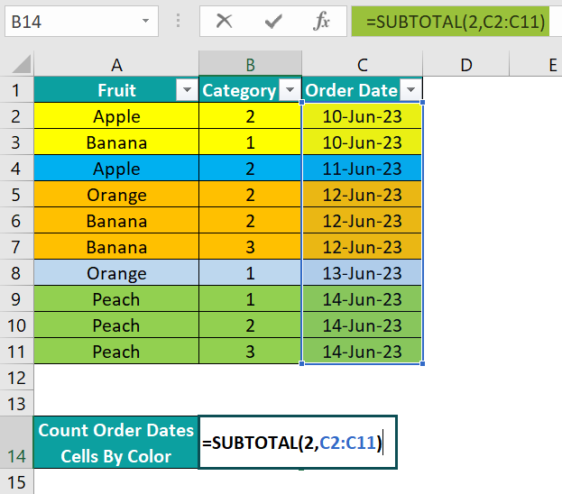
The table below lists fruits, their grades and order dates.

And the rows of data are highlighted in different colors based on the order dates.
Consider the requirement to count the number of cells in column C based on each color and display the output in cell B14.
Then, here is how to use the Filter method with SUBTOTAL() to obtain the output in the target cell.
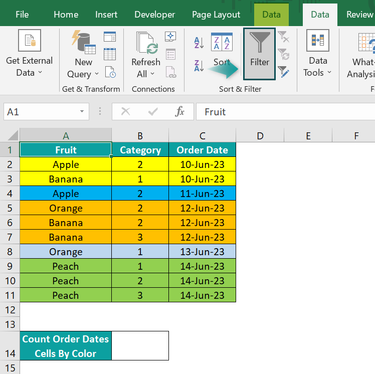
- Step 1: Click in the source dataset and choose Data → Filter or press Ctrl + Shift + L to insert filters in the columns in the dataset.

- Step 2: Choose cell B14 and enter SUBTOTAL()
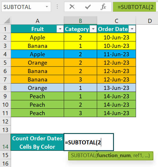
=SUBTOTAL(

Excel will list the options to enter as the first argument, function_num. And as we require to count the number of cells, double-click on the second option, 2 – COUNT, in the drop-down list.
And then enter a comma.
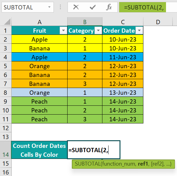
Next, enter the required column cell range from the source dataset and enter the closing bracket, ‘)’.
- Step 3: Press Enter to execute SUBTOTAL() in the target cell B14.
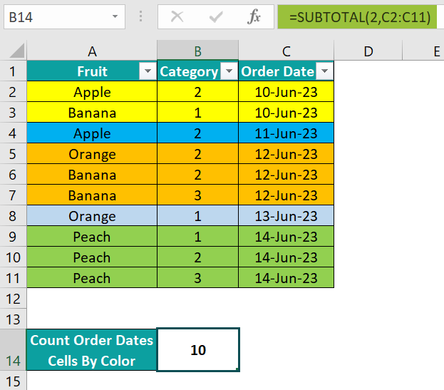
The SUBTOTAL() counts the total number of visible cells in the cell range C2:C11 and returns the output, 10.
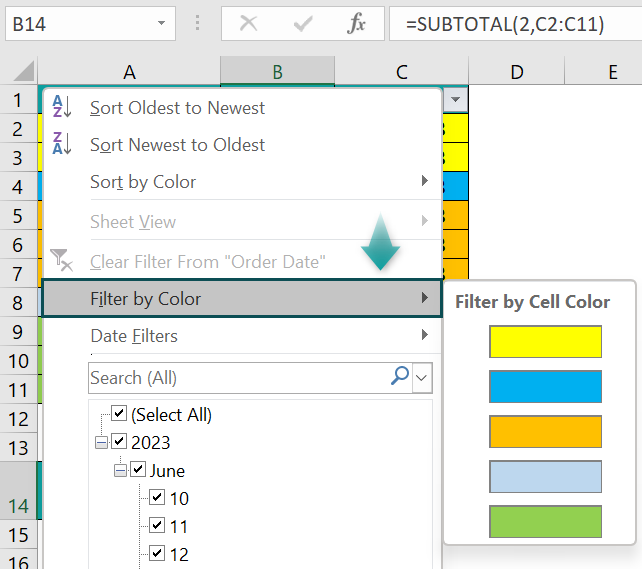
- Step 4: Click the column C filter and select the Filter by Color option from the drop-down list.
- Step 5: Choose the required color, based on which we must count the cells in the chosen range.
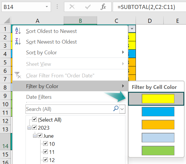
Once we click the required color, the corresponding cells get filtered in the chosen range. And the SUBTOTAL() in cell B14 will return the count of the filtered cells.
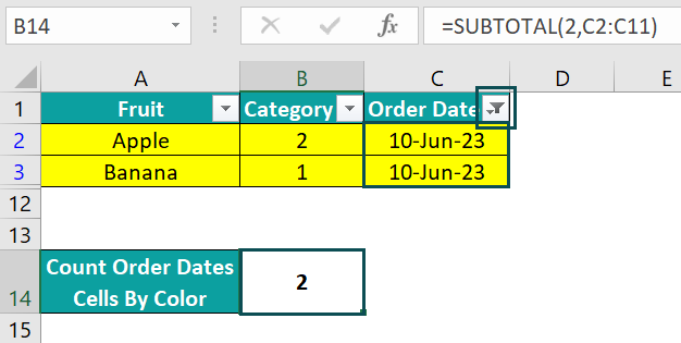
Likewise, we can utilize the Filter option to filter by the required color, one at a time, to count the corresponding number of visible cells in the chosen cell range.
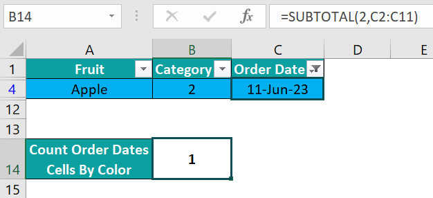
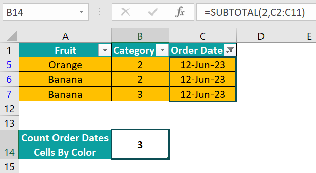

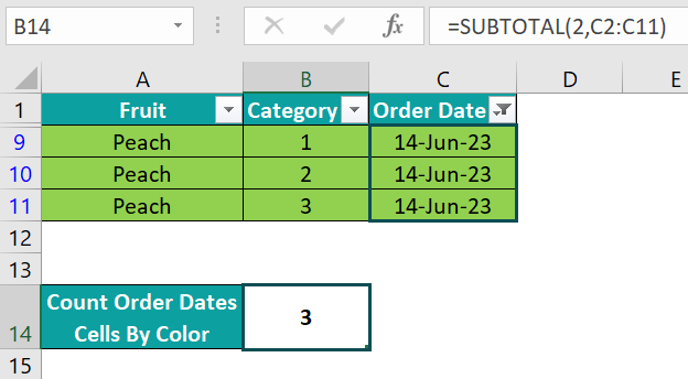
Example #2 – Create Function Using VBA Coding
The first table below shows the annual sales figures for six branch offices of a firm from 2019-22.
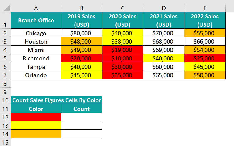
And the sales figures are color-coded based on the different sales ranges.
The requirement is to count cells by color in Excel cell range B2:E7 and display the output for each color in cells B12:B14.
Then, here is how to use VBA coding to achieve the desired result.
- Step 1: With the active worksheet open, use the keys Alt + F11 to open the VBA Editor.

- Step 2: Click Insert → Module to open a new module.

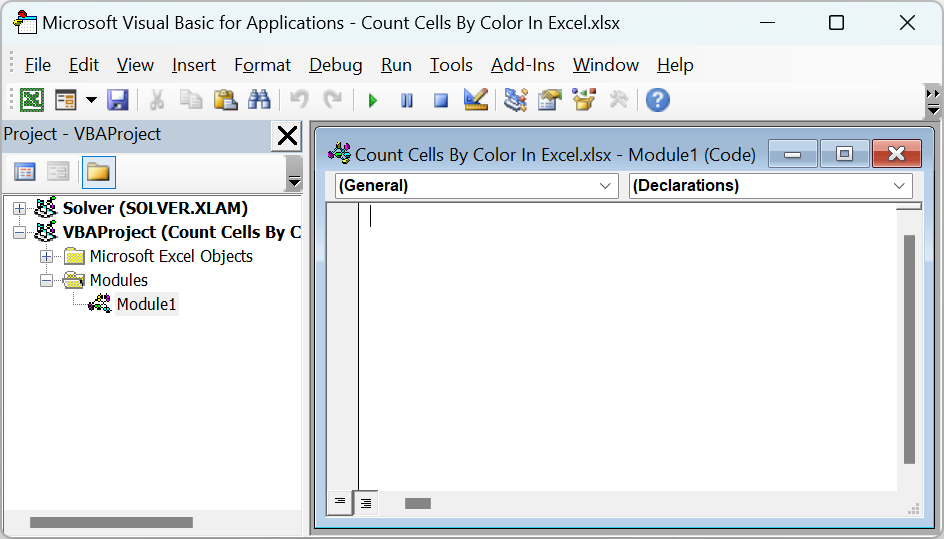
- Step 3: Enter the VBA code in the module to create a user-defined function for counting the cells by the specified color in the chosen cell range.

- Step 4: Select cell B12, enter ‘=’ and COUNT.

Excel will list all the functions starting with COUNT, including VBA functions, where we must double-click the user-defined function created using the VBA coding.
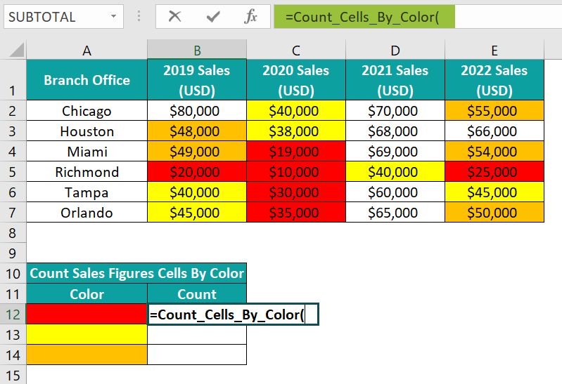
And enter the function arguments, as defined in the VBA code.
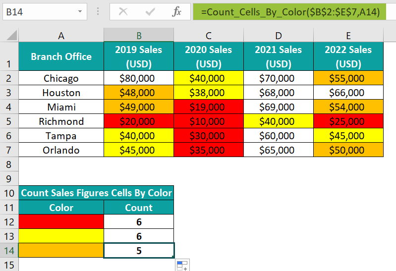
=Count_Cells_By_Color($B$2:$E$7,A12)

We use the Excel absolute reference to the required cell range since the cell range is constant in all the target cells.
- Step 5: Press Enter to view the function output in cell B12, 6.

The function output is the total count of Red cells in the specified cell range.
- Step 6: Using the Excel fill handle, update the formula in the remaining target cells.
The VBA code uses the IF() in a FOR loop, one of the VBA loops, to check each cell in the specified range for the same fill color as the cell containing the required fill color. And the FOR loop counts the matches to return the total number of cells in the cited color.
Important Things To Note
- We can count cells by color in Excel using the SUBTOTAL() when the source cell range lies in one column, and the cells in the specified cell range contain numeric values.
- There is no inbuilt function in VBA to count Excel cells by color. We must write the VBA code to create a user-defined function to count the colored cells across one or more columns with blank and non-empty cells.

Frequently Asked Questions (FAQs)
You can use COUNTIF to count cells by color in Excel.
For example, the first table lists employees, their designations, and pay bands, with each row color-coded based on the designation.
The requirement is to count the column A cells in each color in the second table and display the output in cells B14:B15.
Then, the steps are as follows:
• Step 1: Select cell D2 and choose Formulas → Define Name.
The New Name window opens, where we must update the fields, as shown below.
In this case, we shall utilize the GET.CELL() function in the Refers to field.
Based on the corresponding column A cell, the formula will update the column D cell with the foreground color as a number from 1 to 56. And if the column cell color is automatic (No Fill), the function returns 0.
And click OK.
• Step 2: Enter the newly-created defined name in cell D2.
=COLOR_CODE

And press Enter.
The function output in cell D2 is 36, the cell A2 color code.
• Step 3: Using the fill handle, update the formula in the remaining column D cells, D3:D11.
• Step 4: Select cell B14 and enter the COUNTIF().
=COUNTIF($D$2:$D$11,Color_Code)

And press Enter to execute the function.
• Step 5: Using the fill handle, update the formula in cell B15.
The defined name Color_Code as the second argument in the COUNTIF() returns the foreground color number of the corresponding cell in column A. And then, the COUNTIF() returns the count of the cells in the specified column D cell range containing the foreground color number the second argument returned.
We can count cells by font color in Excel using the following steps:
1) With the active worksheet containing the source dataset open, press Alt + F11 to access the VBA Editor.
2) Choose the required VBAProject and select Insert → Module to open a module window.
3) Enter the following VBA code in the module window to create a user-defined function for counting cells by font color in Excel.
4) Go to the active sheet, select the required target cell and enter the user-defined function with the required argument values.
5) Press Enter to view the function output as the required count of cells by font color in the specified range.
We can count blank cells by color in Excel using the following steps:
1) Open the active worksheet containing the source dataset with blank colored cells and choose Home → Find & Select → Go To Special to open the Go To Special window.
2) Select the Blanks option and click OK.
3) Select Home → Find & Select → Find to open the Find and Replace window.
4) Click Options in the Find tab in the Find and Replace window. And then, choose Format to access the Find Format window.
5) Click the Fill tab to choose the required cell background color based on which we must count the blank colored cells.
6) Click OK in the Find Format window.
7) Click Find All in the Find and Replace window.
Excel will count and list the blank colored cells based on the color specified using the Format button.
Download Template
📥Download the ready-to-use Excel template to practice this tutorial yourself.
Count Cells By Color In ExcelRecommended Articles
This has been a guide to What Is Count Cells By Color In Excel. We learn to do it using Filter method with SUBTOTAL() and VBA coding, with examples. You can learn more from the following articles –

Leave a Reply