Find Errors In Excel

What Is Find Errors In Excel?

The options to find errors in Excel enable one to detect errors, determine their causes, and resolve them to achieve the desired outcome in Excel. We can use the Error Handle error inbuilt functions such as IFERROR to identify and handle an error in a spreadsheet.

Users can find errors in Excel to flag the errors in a sheet so that they can take corrective measures to ensure the Excel data is accurate and more reliable.

For example, the image below shows a dataset containing items and their quantities, with the average quantity per item calculated in cell B13 based on cell range B2:B11 data.

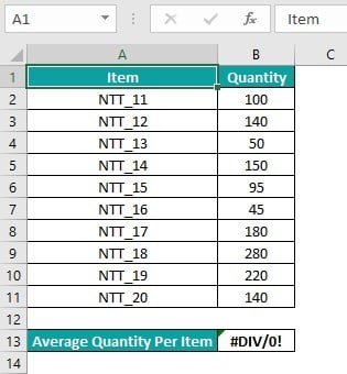
However, cell B13 shows the output as an error value, #DIV/0!.

Here is how to use the Error Handler, which helps find and replace errors in Excel.

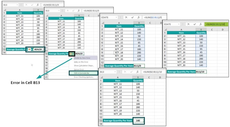
In the above find and replace errors in Excel example, we first select cell B13.

The Warning icon (a Yellow diamond with the Exclamation Mark) will appear on the left of the chosen cell. Next, we click the warning icon drop-down arrow to find the error in the chosen cell, which will be the first entry in the drop-down list.

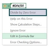
In this case, the first entry in the drop-down list indicates a divide by zero error, which helps us decide on further action to resolve the issue.

So, we choose the Edit in Formula Bar option from the drop-down list and correct the cell B13 formula in the Formula Bar by updating the denominator value as 10. Finally, pressing Enter will execute the cell B13 formula, and we will achieve the correct output.

How To Find Errors In Excel?

We can find errors in Excel using the following methods:

1. Using Error Handler
2. Using Error Checking Option
3. Using Go To Special Option To Find Errors Due To Formulas

Method #1 – Using Error Handler

This method uses the Error Handler, represented by the Warning icon (a Yellow diamond with the Exclamation Mark), to find the error in a specific cell.

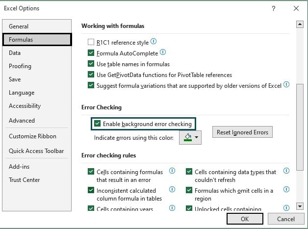
But first, we must enable the background error-checking option in the Excel Options window to view and use the Error Handler.

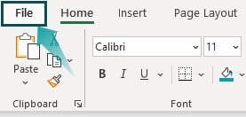
• Open the required Excel workbook, choose the File tab and select the Options option.

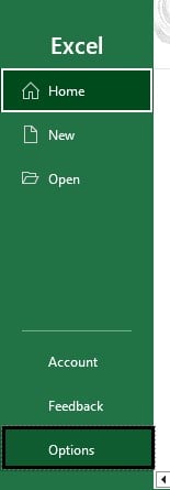
• The Excel Options window will open, where we must click the Formulas tab to open it. Next, check the Enable background error checking option checkbox in the Error Checking section and click OK to close the window.

Once we enable the specified option in the Excel Options window, Excel will show a small Green triangle at the top-left corner of a cell containing an error value.

For instance, the below image shows a cell containing the #DIV/0! Excel error value, with the Green triangle visible in the cell.

Next, choosing the above cell will show the Error Handler next to the cell as the Warning icon.

We can hover the mouse cursor on the Warning icon to access its drop-down arrow.

Also, hovering the cursor over the Warning icon will show a hovering message stating the error in the specific cell.

Finally, clicking the Warning icon drop-down arrow will open a drop-down list, with the first entry specifying the error in the chosen cell.

While this method helps locate errors due to incorrect formulas, such as the find REF errors in Excel, we can also find errors due to incorrect data formats.

Method #2 – Using Error Checking Option

Consider the background error checking option in the Excel Options window is unchecked.

Then, the Green triangle, explained in the previous section, will not be visible, even if a cell shows an error value.

In such a scenario, we can use the Error Checking option in the Formulas tab as explained below:

• Open the worksheet, where we aim to find the errors.
• Choose the Formulas tab – Error Checking option down arrow – Error Checking option.

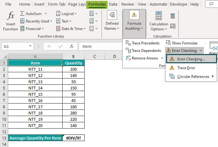
• The first cell with an error will appear selected in the sheet. Simultaneously, the Error Checking window will open, where we can find the reference to the chosen cell containing the error value and the corresponding error explanation.

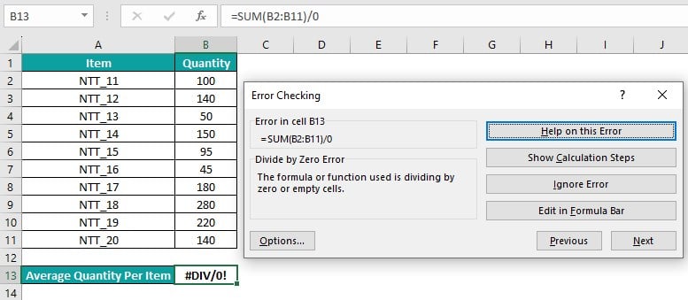
Furthermore, if we must check the worksheet for more errors, click Next to find the next cell with an error value. The next cell containing the error will be selected if the sheet has more cells with error values. Otherwise, Excel will show a message box indicating the error checking is complete for the sheet.

Also, we can select Previous and Next to navigate between the cells containing errors in the specific sheet.

Finally, click OK in the message box to close the box and the Error Checking window.

Thus, we can find multiple errors in a worksheet, one at a time, using the Error Checking option.

[Alternatively, open the worksheet, where we must find the errors. Next, use Alt + M + K + K as the shortcut to find errors in Excel since using the specified key combination will open the Error Checking window. Next, follow the above steps to complete the error-finding process once the Error Checking window opens.]

Method #3 – Using Go To Special Option To Find Errors Due To Formulas

This method finds multiple cells containing error values due to formulas in one go. Also, we assume the background error-checking option in the Excel Options window is checked.

The steps to find errors in a sheet using the Go To Special option are as follows:

• Open the sheet where we must find the errors.
• Choose the Home tab – Find & Select option down arrow – Go To Special option.

• The Go To Special window will open, where we must choose the Formulas option, under which the Errors option checkbox will be checked.

[Alternatively, we can open the worksheet, where we must find the errors. Then, use Alt + H + FD + S + F as the shortcut to find errors in Excel. It is because the specified keys combination will open the Go To Special window and select the Formulas radio button, under which the Errors option will appear selected.]

• Press OK to close the window and view all the cells containing the error values due to formulas in the specific sheet, highlighted in one go.
• Next, select a highlighted cell to enable the Error Handler and access the Warning icon drop-down list to find the error in the chosen cell.
• Repeat step 5 to find the error in the next highlighted cell.

How To Handle Errors In Excel?

Once we find errors in Excel, we can handle them using the following methods:

1. Error Handling Through Error Handler
2. Formulas Error Handling

Method #1 – Error Handling Through Error Handler

The steps to handle errors through Error Handler are as follows:

1. Select the cell where we found the error.
2. Assuming the background error-checking option is checked in the Excel Options window, the Error Handler (warning icon) will appear on the left side of the chosen cell.
3. Hover the mouse cursor on the Error Handler to access it drop-down arrow.
4. Once we click the drop-down arrow, the drop-down list opens, listing the possible options to resolve the error based on the error specified in the first entry in the list.
5. Choose the applicable option from the drop-down list, probably the second entry, to proceed with the error-handling process.

Method #2 – Formulas Error Handling

While the previous method helps correct errors due to incorrect data formats, we can also resolve errors due to incorrect formulas. For instance, we can find REF errors in Excel and eliminate them.

But first, we must know the possible error values Excel formulas return.

Error Value	Description
#DIV/0!	The error occurs when the number is divided by zero or empty cells.
#NAME?	The error occurs when Excel does not recognize the function name.
#N/A	The error occurs when the VLOOKUP() does not find the search value in the specified lookup range.
#REF!	The error occurs when the cell referenced in the formula is deleted, or the reference area specified in the formula is out of range.
#VALUE!	The error occurs when the data types included in the formula are incorrect.

So, here is how to proceed with formulas error handling:

1. Select the cell containing the error due to the formula entered into it.
2. Rewrite the formula by entering =IFERROR( in the chosen cell. [ Alternatively, type =IF or =IFE to choose Excel IFERROR function from the suggestions.]
3. Let the formula, previously existing in the chosen cell, be the first argument, value. Next, enter a comma, and the second argument, value_if_error, will be the value we wish to display in the chosen cell instead of the error value.
4. Close the bracket and press Enter to execute the IFERROR() and overcome the error in the chosen cell.

Examples

The following examples explain how to find errors in Excel and handle them effectively.

Example #1 – Error Handling Through Error Handler

The following dataset contains a list of students and their Mathematics test scores.

However, the cells containing the Mathematics test scores, B2:B11, appear to have errors.

Thus, here is how to find and handle errors in the current sheet.

Step 1: Choose cell B2. We can view the Error Handler to the left of the chosen cell.

Next, hover the mouse cursor over the Error Handler to view the hovering message stating the error in the chosen cell.

Step 2: We can choose the remaining cells B3:B11 to check the errors in each cell, as explained in Step 1, individually.

So, we find that all the cells B2:B11 have the same error.

In such a scenario, we can choose the entire cell range B2:B11 to view the Error Handler for all the chosen cells on the left of the first cell in the selection.

Step 3: Place the mouse cursor on the Error Handler and click the Warning icon’s drop-down arrow.

The drop-down list opens, where the first entry explains the error, again helping us find the error in the chosen cells.

In this example, the test scores in cells B2:B11 are numbers. But they are stored as text values. So, we choose the second option in the drop-down list, Convert to Number, to remove the errors in the chosen range.

[Alternatively, with the sheet containing the source dataset open, choose Formulas – Error Checking down arrow – Error Checking.

The first cell containing an error, cell B2, gets selected, and the Error Checking window opens, explaining the error in the chosen cell.

In this example, the error is due to the incorrect data format. So, choose the Convert to Number option in the Error Checking window to remove the error in the chosen cell B2.

Next, once we click the Convert to Number option, the Error Checking window shows the error explanation for the next cell containing the error in the worksheet. We can choose the Convert to Number option to remove the error in the specific cell.

Likewise, repeat the process for all the cells containing the error.

Finally, once the last cell containing the error gets selected, click the Convert to Number option.

Next, Excel will show a message stating that the error check is complete for the entire worksheet. We can click OK to close the box and window and view an error-free sheet.

Please note that the option provided in the Error Checking window to handle the error will depend on the error type to resolve.

Example #2 – Formulas Error Handling

The following image shows two datasets.

The first dataset in the cell range A1:D11 contains an employees list, their designations, projects, and appraisal statuses. On the other hand, the second dataset shows the appraisal status of the employee specified in cell F2, using the Excel VLOOKUP function in cell G2 based on the first dataset.

However, the VLOOKUP() output is an error. Then, here is how to find the error definition and handle the error in cell G2.

Step 1: Since cell G2 is already selected, the Error Handler is visible.

So, hover the mouse cursor over the Error Handler to select the Warning icon’s drop-down arrow and check the error in cell G2 from the drop-down list.

In this example, the error in the Warning icon drop-down list, Value Not Available Error, indicates that the lookup value, Kevin Reed, is not present in the lookup range, A2:D11. Hence, the function does not get the required return value in the source dataset and returns the #N/A error as the output.

Step 2: Choose cell G2 and enter the following IFERROR().

=IFERROR(VLOOKUP(F2,A2:D11,4,0),”Data Not Available”)

Step 3: Press Enter to view the formula output.

First, the VLOOKUP() searches for the lookup value, Kevin Reed, in the lookup range A2:D11. Since the first column in the lookup range does not contain the lookup value, the function cannot determine the return value and returns the #N/A error value.

Next, the IFERROR() accepts the VLOOKUP() output as the first argument. And since the VLOOKUP() output is an error value, the IFERROR() replaces the error value in cell G2 with the phrase supplied as the second argument, Data Not Available.

Thus, the IFERROR() helps handle errors due to formulas in Excel.

Important Things To Note

• Enable the background error-checking option in the Excel Options window to use the Error Handler to find errors in Excel.
• A cell will show the error notifier, the Green triangle, on the upper-left corner of the cell if the cell data format is incorrect or the cell contains a formula returning an error value.
• The Go To Special option is useful only when we must find errors in Excel due to formulas.

Frequently Asked Questions (FAQs)

Download Template

This article must be helpful to understand the Find Errors In Excel, with its formula and examples. You can download the template here to use it instantly.

Recommended Articles

This has been a guide to What Is Find Errors In Excel. We explain the ways to find errors and handle them in Excel, with examples and points to remember. You may learn more from the following articles –

• Error Bars In Excel
• #DIV/0! Excel Error
• #VALUE! Error In Excel