
What Is IFS Function In Excel?
The IFS Excel function helps users provide multiple conditions and returns TRUE when the first TRUE condition is met. This function is an alternative for the Nested IF function.
The IFS function in Excel is an inbuilt Logical function, so we can insert the formula from the “Function Library” or enter it directly in the worksheet.
Use this IFS Excel Function Template to follow along with the examples in this article.
Download Excel TemplateFor example, we will apply the IFS function to calculate the output for the following data.

Select cell B2, enter the formula =IFS(A2=10,TRUE), and press the “Enter” key.

The result is ‘TRUE’, as shown above.
Key Takeaways
- The IFS Excel function checks if the selected cells fulfills all the provided conditions or criteria. Then, it returns the corresponding values when it gets the first true test condition.
- Two main arguments of the function are “logical_test”, and “value_if_true”, then for multiple conditions, the formula is entered as “logical_test1,value_if_true1,[ logical_test2,value_if_true2],[ logical_test3,value_if_true3],……and so on”, up to 127 conditions.
- The function is an alternative for the IF…Else or the nested IF functions, which are easy to work on by avoiding errors like missing out on brackets, conditions, etc.
IFS() Excel Formula
The syntax of the IFS Excel formula is,

The arguments of the IFS Excel formula are,
- logical_test1: It is a mandatory argument. It is the first test condition used to evaluate whether the test condition is TRUE or FALSE.
- value_if_true1: It is a mandatory argument. The result is returned when the logical_test1 condition is true. The value of this argument can be kept blank or empty.
How To Use IFS Excel Function?
We can use the IFS Excel function in 2 ways, namely,
- Access from the Excel ribbon.
- Enter in the worksheet manually.
Method #1 – Access from the Excel ribbon
Choose an empty cell for the output → select the “Formulas” tab → go to the “Function Library” group → click the “Logical” option drop-down → select the “IFS” function, as shown below.

The “Function Arguments” window appears. Enter the arguments in the “Logical_test”, and the “Value_if_true” fields → click “OK”, as shown below.

Method #2 – Enter in the worksheet manually
- Select an empty cell for the output.
- Type =IFS( in the selected cell. [Alternatively, type =I and double-click the IFS function from the list of suggestions shown by Excel.]
- Enter the arguments as cell values or excel cell references and close the brackets.
- Press the “Enter” key.
Let’s take a basic example to learn its application.
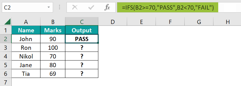
We will calculate pass or fail using IFS Excel function for the name of the students and their marks.
In the table, the data is,
- Column A contains the Name.
- Column B contains the Marks.
- Column C contains the Output.

The steps to calculate the value using IFS formula are,
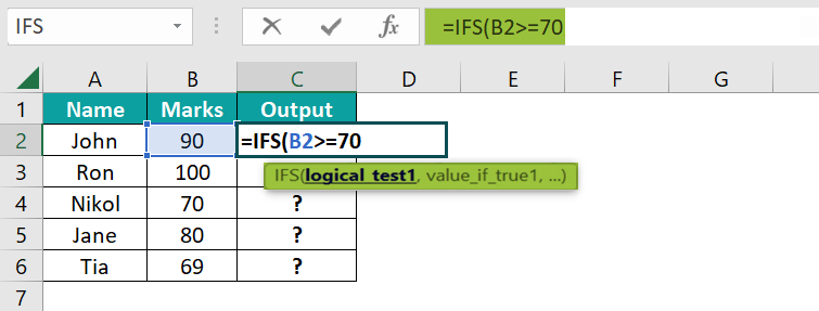
- Select cell C2, and enter the formula =IFS(B2>=70, i.e., the test condition value.
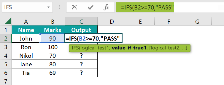
- Enter the value of ‘value_if_true1’ as “PASS,” i.e., the result value. The formula is now =IFS(B2>=70,”PASS”
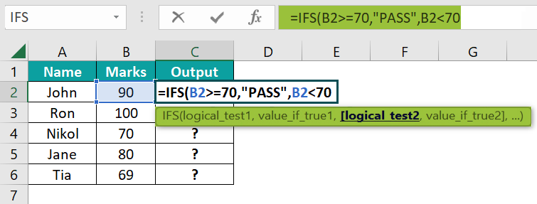
- Enter the value of ‘logical_test2’ as B2<70, i.e., the second test condition value. The formula now is =IFS(B2>=70,”PASS”,B2<70
- Enter the value of ‘value_if_true2’ as “FAIL”, i.e., the second conditions result value, and close the brackets. The complete formula is =IFS(B2>=70,”PASS”,B2<70,”FAIL”).
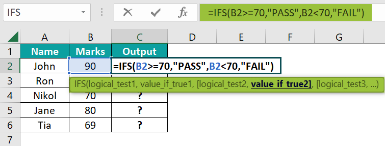
- Press the “Enter” key. The result is “PASS”, as shown below.
- Drag the formula from cell C2 to C6 using the fill handle.
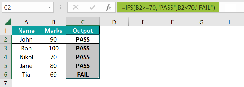
The output is shown above. The formula checks for multiple conditions, i.e., B2>=70 and B2<70, if the scores are greater than or equal to 70, then the results are PASS, as displayed in cells C2 to C5, and if the scores are less than 70, then the result is FAIL, as displayed in cell C6.
Examples
We will understand some advanced scenarios using the IFS Excel function examples.
Example #1
We will calculate the status using the IFS function for the fruits and their amount in stock.
- In the table, the data is,
- Column A contains the Fruits.
- Column B contains the Amount in Stock.
- Column C contains the Status.

The steps to calculate the value using the IFS formula are,
- Step 1: Select cell C2, enter the formula =IFS(B2<=20,”Order”,B2>20,”Full”), and press “Enter”. The result is “Order”, as shown below.
[Note: ‘logical_test1’ as B2<=20, ‘value_if_true1’ as “Order”, ‘logical_test2’ as B2>20, and ‘value_if_true2’ as “Full”.]

- Step 2: Drag the formula from cell C2 to C9 using the fill handle. The output is shown below.

Example #2
We will calculate the status using the IFS function for the companies and their turnover.
In the table, the data is,
- Column A contains the Company.
- Column B contains the Turnover.
- Column C contains the Status.

The steps to calculate the value using the IFS formula are,
- Step 1: Select cell C2, enter the formula =IFS(B2>400000,”Excellent Turnover”,B2<400000,”Average”), and press “Enter”. The result is “Excellent Turnover”, as shown below.
[Note: ‘logical_test1’ as B2>400000, ‘value_if_true1’ as “Excellent Turnover”, ‘logical_test2’ as B2<400000, and ‘value_if_true2’ as “Average”.]

- Step 2: Drag the formula from cell C2 to C6 using the fill handle. The output is shown below.

Example #3
We will calculate the deduction rate according to the slab using the IFS function for the name of the employees and annual salary.
In the table, the data is,
- Column A contains the Name.
- Column B contains the Annual Salary.
- Column C contains the Deduction.

The steps to calculate the value using the IFS formula are,
- Step 1: Select cell C2, enter the formula =IFS(B2<300000,”6%”,B2>300000,”8%”), and press “Enter”. The result is “6%”, as shown below.
[Note: ‘logical_test1’ as B2<300000, ‘value_if_true1’ as “6%”, ‘logical_test2’ as B2>300000, and ‘value_if_true2’ as “8%”.]

- Step 2: Drag the formula from cell C2 to C6 using the fill handle. The output is shown below.

Important Things To Note
- The “#N/A” error occurs when the IFS function finds no TRUE conditions.
- The “#VALUE!” error occurs when the “logical_test” argument solves to a value other than TRUE or FALSE.
- The “You’ve entered too few arguments for this function” error message appears when the “logical_test” argument is entered without a corresponding value.
Frequently Asked Questions (FAQs)
The IFS function checks multiple conditions and returns a value corresponding to the first TRUE condition.
The syntax of theIFS function is =IFS(logical_test1,value_if_true1,[ logical_test2,value_if_true2],… )
We can insert the IFS function as follows:
1. Select an empty cell for the output.
2. Type =IFS( in the selected cell. [Alternatively, type =I and double-click the IFS function from the list of suggestions shown by Excel.]
3. Enter the arguments as cell values or cell references and close the brackets.
4. Press the “Enter” key.
For example, we will calculate that output using the IFS function for some values.
In the table, the data is,
• Column A contains the Value.
• Column B contains the Output.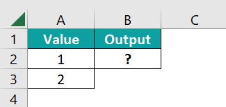
The procedure to calculate the value using the IFS formula is,
Select cell B2, enter the formula =IFS(A3<A2,TRUE), and press the “Enter” key.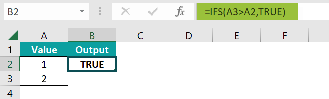
The result is “TRUE”, as shown above.
The IFS function is found in the “Formulas” tab, as shown below.
Choose an empty cell for the output → select the “Formulas” tab → go to the “Function Library” group → click the “Logical” option drop-down → select the “IFS” function, as shown below.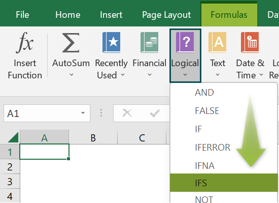
Use this IFS Excel Function Template to follow along with the examples in this article.
Download Excel TemplateRecommended Articles
Continue with these related resources when you want the next practical step in this topic.
- IF Function In Excel
- Logical Operators in Excel
- Logical Test In Excel
- AND Function in Excel
- OR Function In Excel
Explore the full Excel Logical Functions guide or browse Excel Resources.