AVERAGEIFS Excel Function

What Is AVERAGEIFS Function In Excel?

The AVERAGEIFS Function in Excel calculates the average/mean of the numeric values that match multiple criteria given for a selected dataset. The logical operators (>,<,<>,=) and wildcards (*,?) can be used by the AVERAGEIFS function just like the SUMIFS and COUNTIFS functions. The AVERAGEIFS Excel function is an inbuilt Statistical function, so we can insert the formula from the “Function Library” or enter it directly in the worksheet.

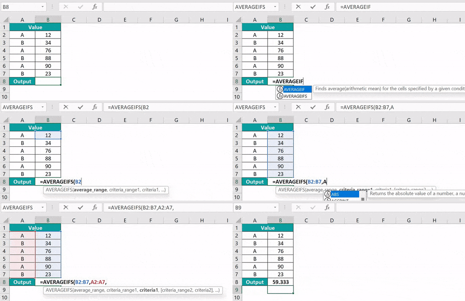
For example, the following image shows values in columns A and B. We will calculate the average of the numbers based on set criteria using the AVERAGEIFS Excel function.

Select cell B8, enter the formula =AVERAGEIFS(B2:B7,A2:A7,”A”), and press “Enter”. The result is ‘59.333’, as shown below.

AVERAGEIFS() Excel Formula

The syntax of the AVERAGEIFS Excel formula is,

The arguments of the AVERAGEIFS Excel formula are,

• average_range: It is a mandatory argument. It is the cell rage to find the average.
• criteria_range1: It is a mandatory argument. It is a cell range to apply the criteria.
• criteria1: It is a mandatory argument. It is the first criteria for the first cell range from the given dataset, followed by [criteria_range2,criteria2], [criteria_range3,criteria3], and so on…

How To Use AVERAGEIFS Excel Function?

We can use the AVERAGEIFS function in Excel in two ways, namely,

1. Access from the Excel ribbon.
2. Enter in the worksheet manually.

Method #1 – Access from the Excel ribbon

Choose an empty cell for the output → select the “Formulas” tab → go to the “Function Library” group → click the “More Functions” option drop-down → click the “Statistical” option right arrow → select the “AVERAGEIFS” function, as shown below.

The “Function Arguments” window appears. Enter the arguments in the “Average_range”, “Criteria_range1”, and “criteria” fields → click “OK”, as shown below.

[Note: To view the “Criteria1” field, click the “Criteria_range1” field.]

Method #2 – Enter in the worksheet manually

1. Select an empty cell for the output.
2. Type =AVERAGEIFS( in the cell. [Alternatively, type =A and double-click the AVERAGEIFS function from the Excel suggestions.]
3. Enter the arguments as cell values or cell references in Excel.
4. Close the brackets of the formula.
5. Press the “Enter” key.

Let us take a basic example to understand this function.

Here, we will calculate the average of the numbers based on set criteria using AVERAGEIFS Excel function for the zonal-wise employee sales.

In the table, the data is,

• Column A contains the Zone.
• Column B contains the Employee.
• Column C contains the Sales.

Examples

We will understand some advanced scenarios using AVERAGEIFS Excel function examples.

Example #1

We will calculate the average of the numbers based on set criteria using the AVERAGEIFS function for the product quantity.

In the table, the data is,

• Column A contains the Product.
• Column B contains the Quantity.

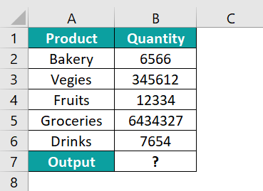
The procedure to calculate the average using the AVERAGEIFS Excel function is,

Select cell B7, enter the formula =AVERAGEIFS(B2:B6,A2:A6,”Bakery”), and press the “Enter” key.

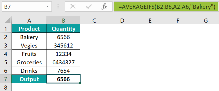
The result is “6566”, as shown above.

Example #2

We will calculate the average of the numbers based on set criteria using AVERAGEIFS Excel function for the student marks.

In the table, the data is,

• Column A contains the Class.
• Column B contains the Marks.

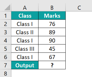
The procedure to calculate the average using the AVERAGEIFS Excel function is,

Select cell B7, enter the formula =AVERAGEIFS(B2:B6,A2:A6,”Class I”), and press the “Enter” key.

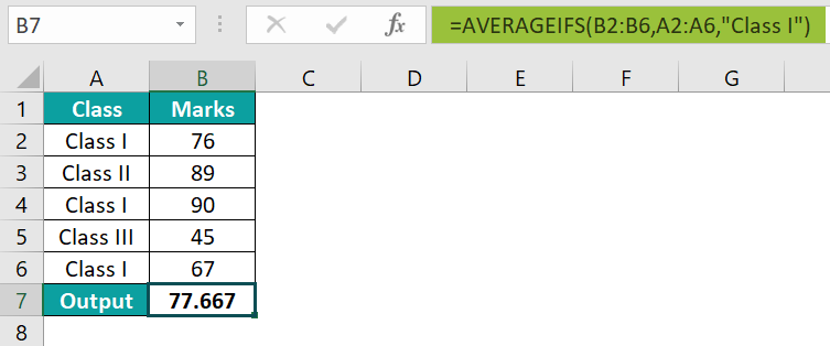
The result is “7.667”, as shown above.

Example #3

We will calculate the average of the numbers based on multiple criteria using the AVERAGEIFS formula for the medals won by countries in the tennis tournament, and

In the table, the data is,

• Column A contains the Countries.
• Column B contains the Result.
• Column C contains the Medals.

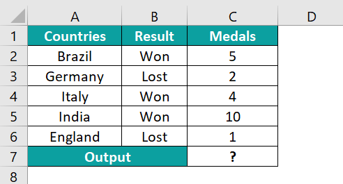
The steps to calculate the average with multiple criteria using the AVERAGEIFS Function are,

• Step 1: Select cell C7, enter the formula =AVERAGEIFS(C2:C6,B2:B6,”Won”  

[Note: The first criteria, i.e., criteria1, is to check for “Won” in the criteria_range1, B2:B6.]

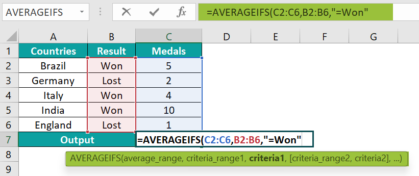
• Step 2: In continuation with the formula, select the criteria_range2, A2:A6, and the second criteria, i.e., criteria2 as *a*, which will check for the country names having the letter ‘a’, and close the brackets.

Therefore, the complete formula is =AVERAGEIFS(C2:C6,B2:B6,”=Won”,A2:A6,”*a*”) 

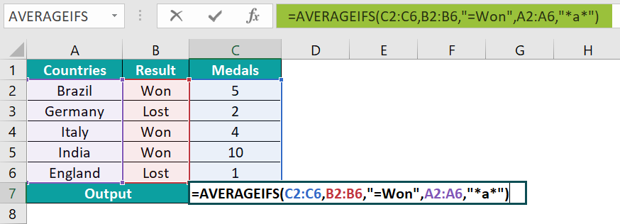
• Step 3: Press the “Enter” key.

The result is “6.333333333”, as shown above.

[Output Observation: The formula first checks whether cell range C2:C6 satisfies both conditions.

• Condition 1: The cells C2, C4, and C5, have the text string “Won” in their cells B2, B4, and B5, respectively.
• Condition 2: Their respective countries in cells A2, A4, and A5, i.e., Brazil, Italy, and India, have the letter ‘a’ in their names.

Therefore, the cell values that satisfy both conditions are C2, C4, and C5. Now, the formula calculates the average,i.e., (C2+C4+C5)/3, which is (5+4+10)/3 or 19/3=6.33333.]

Important Things To Note

• The “#DIV/0!” error occurs when:
  • The “average_range” argument is left blank or is a text value.
  • None of the criteria are met.
• Each “criteria_range” provided in the formula must be the same size, else we will get the “#VALUE!” error.
• We will get a “#NAME?” error if the function’s name is incorrectly entered in the formula or if we do not close the brackets of the formula.  

Frequently Asked Questions (FAQs)

Download Template

This article must help understand the AVERAGEIFS Excel function, with its formula and examples. You can download the template here to use it instantly.

Recommended Articles

This has been a guide to AVERAGEIFS Excel Function. Here we explain how to use AVERAGEIFS formula along with examples & downloadable excel template. You can learn more from the following articles –

• AVERAGEIF Function in Excel
• Weighted Average In Excel
• AVERAGE Excel Function