What Is Lookup Table In Excel?
A lookup table in Excel is a table that contains a lookup value and its return value. And we can create an Excel lookup table using the inbuilt functions VLOOKUP, LOOKUP, and INDEX-MATCH.
Users can utilize an Excel lookup table when the requirement is to locate the data associated with a value in a massive dataset.
For example, the first table in the following image lists students and their overall percentages and grades.
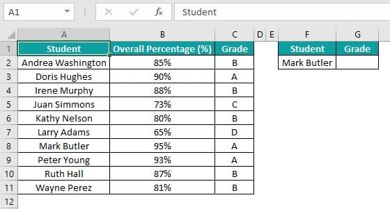
The task is to look up a student’s name in the source dataset and update their grade.
Then, in such a scenario, we can use a lookup table in Excel based on the Excel LOOKUP function to achieve the required output.
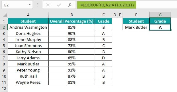
In the above lookup table in Excel example, we shall create the required lookup table in the cell range F1:G2.
While the lookup value is in cell F2, we use the Excel LOOKUP function in cell G2 to search for the specified lookup value in the lookup vector range A2:A11. And then, the function returns the value from the same row of the result vector range, C2:C11, as the lookup value.
Furthermore, we can change the lookup value in cell F2. And the LOOKUP() in cell G2 will automatically return the updated output in the lookup table.
Table of contents
Key Takeaways
- The lookup table in Excel is a cell range containing a lookup value and a return value based on the specified dataset.
- Users can use the Excel lookup table to check for a value in a large dataset in the same or different worksheet or workbook to obtain the corresponding data.
- We can use the inbuilt functions VLOOKUP, LOOKUP, and INDEX-MATCH, to define an Excel lookup table.
- We can use the abovementioned functions with other inbuilt functions, such as IF, to create lookup tables for more practical results.
How To Create A Lookup Table In Excel?
We can create or insert lookup table in Excel using the following methods:
- Create a Lookup Table Using VLOOKUP Function
- Use LOOKUP Function to Create a LOOKUP Table in Excel
- Use INDEX + MATCH Function
Let us see the steps with a lookup table in Excel example for each method.
#1 – Create A Lookup Table Using VLOOKUP Function
The steps to create an Excel lookup table using the VLOOKUP() are as follows:
- Choose a cell range to build a lookup table.
- Update the lookup table column headings.
- Enter the lookup value in the second cell of the first column.
- Choose the second cell in the second column as the target cell to display the output.
- Type =VLOOKUP( in the target cell. [Alternatively, type =V or =VL and choose the VLOOKUP function from the Excel suggestions.]
- Enter the Excel VLOOKUP function argument values, separated by commas. And then close the bracket.
The VLOOKUP() syntax is as follows:

Where,
- lookup_value: The value we aim to look up.
- table_array: The range in which the function must search the lookup value and the corresponding return value.
- col_index_num: The number of the column in the table_array range containing the required output, the return value.
- range_lookup: The logical value indicating whether the function must find an approximate or exact match as the return value.
While the first three arguments are mandatory, the fourth is optional.
7. Press Enter to view the required output in the lookup table.
Basic Example
The table below shows a firm’s invoice data.
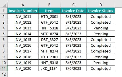
The task is to insert lookup table in Excel cell range G1:H2 to look up the invoice number in the source dataset to determine the invoice status.
Then, here is how to use the VLOOKUP() to build a lookup table in the target cell range.
Step 1: Choose cell G1 and enter the first column heading in the lookup table. Next, select cell H1 and enter the second column heading in the lookup table.
And then, choose cell G2 and enter the lookup value.
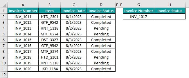
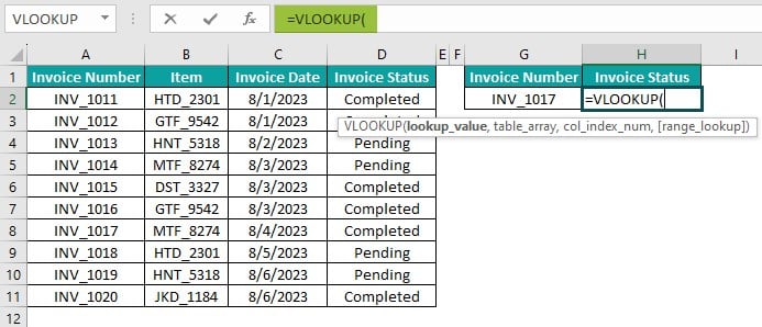
Step 2: Choose cell H2 and enter the VLOOKUP() to use a lookup table in Excel cell range G1:H2 and display the output.
=VLOOKUP(
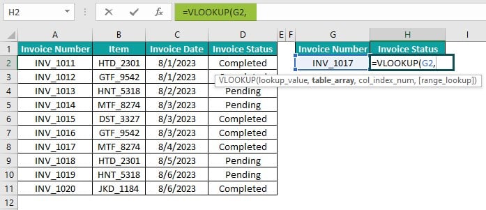
Next, enter the excel cell reference to the given lookup value, followed by a comma.
=VLOOKUP(G2,
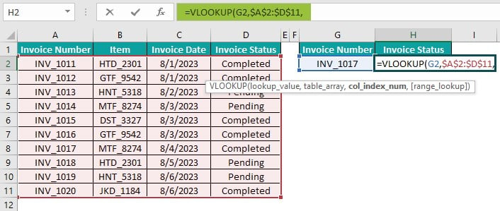
And then, enter the Excel absolute reference to the lookup range, A2:D11, followed by a comma.
=VLOOKUP(G2,$A$2:$D$11,
Next, enter the column number containing the return value, 4, followed by a comma.
=VLOOKUP(G2,$A$2:$D$11,4,

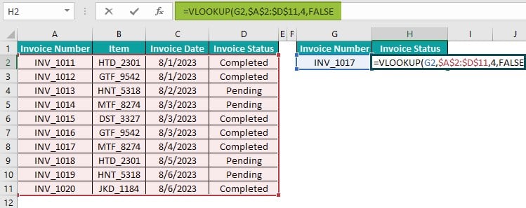
And then, Excel shows the logical values of the last argument, TRUE and FALSE.
We shall double-click FALSE to choose it, as we want an exact match to obtain the required return value.
=VLOOKUP(G2,$A$2:$D$11,4,FALSE
Finally, enter the closing bracket.
=VLOOKUP(G2,$A$2:$D$11,4,FALSE)
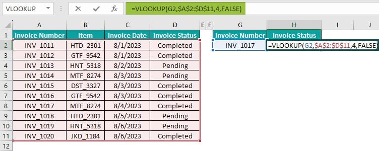
Step 3: Press Enter to view the VLOOKUP() output in cell H2.
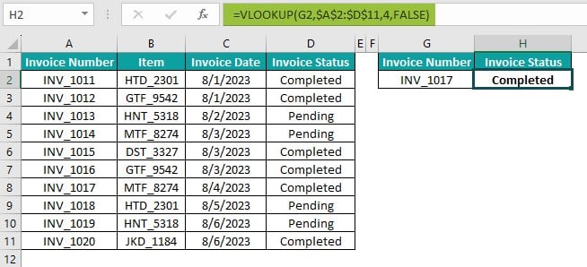
Next, we can change the lookup value in cell G2 to edit lookup table in Excel cell range G1:H2.
However, a more sophisticated option is to create a drop-down list in cell G2 to enable the user to choose the lookup value from the list rather than changing the value manually.
And for that, we can use the Excel Data Validation feature from the Data tab.
Step 4: Select cell G2 and Data tab – Data Validation function – Data Validation option.
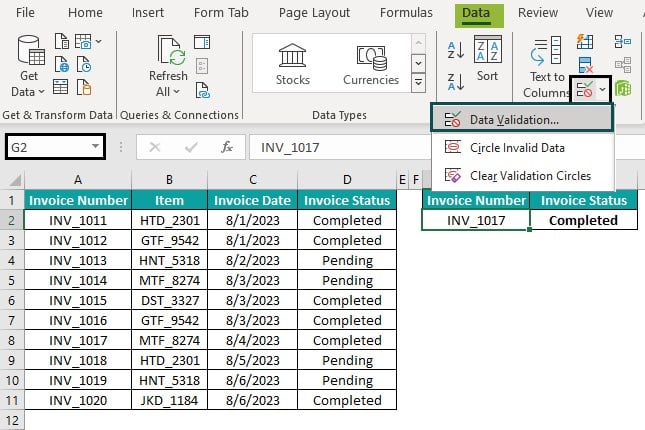
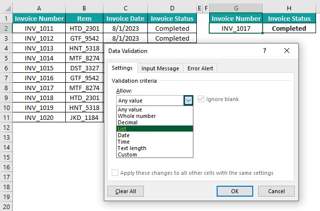
The Data Validation window will open.
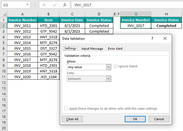
Step 2: Click the Allow field drop-down button to set the field as List.
Next, update the first column data range of the lookup range where the VLOOKUP() must search for the lookup value in the Source field.
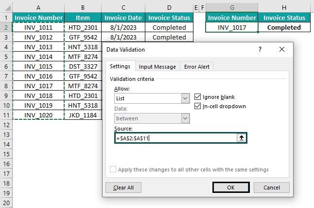
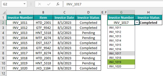
And click OK in the Data Validation window to close it and view the drop-down button in cell G2.

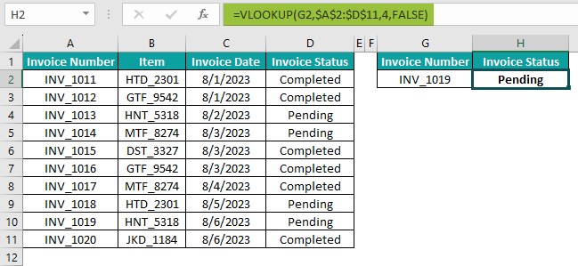
Now, we can edit lookup table in Excel by changing the lookup value in cell G2 using its drop-down button and list. Accordingly, the VLOOKUP() in cell H2 will show the updated return value.
#2 – Use LOOKUP Function To Create A LOOKUP Table In Excel
The steps to use LOOKUP() to create an Excel lookup table are as follows:
- Select a cell range to display a lookup table.
- Enter the lookup table column headings.
- Update the lookup value in the second cell of the first column of the lookup table.
- Choose the second cell in the second column as the target cell to display the output.
- Type =LOOKUP( in the target cell. [ Alternatively, type =LO and choose LOOKUP from the Excel suggestions.]
- Enter the LOOKUP() argument values, separated by commas. And then close the bracket.
The LOOKUP() syntax is as follows:

Where,
- lookup_value: The value we must look up in the lookup_vector.
- lookup_vector: The cell range containing a single row or column in which the function must search the lookup value.
- result_vector: A cell range containing a single row or column. And it is the same size as the lookup_vector.
While the first two arguments are mandatory, the third is optional.
7. Press Enter to obtain the required output in the lookup table.
Basic Example
The following table lists US states and their population statistics.
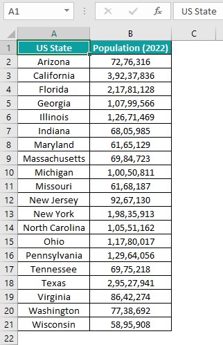
The requirement is to define an Excel lookup table in the cell range F1:G2 to look up a US state name and display its population.
Then, we can create an Excel lookup table in the target cell range using the LOOKUP().
Step 1: Choose cell F1 and enter the heading of the first column in the lookup table. Next, select cell G1 and enter the heading of the second column in the lookup table.
And then, choose cell F2 and enter the required lookup value.
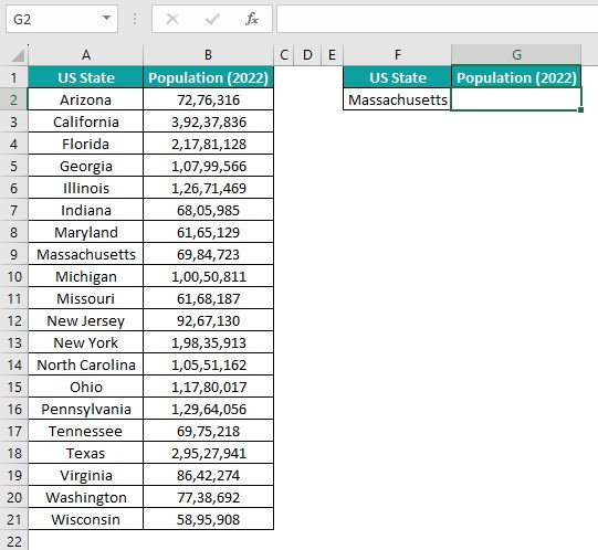
Step 2: Choose cell G2 and enter the LOOKUP().
=LOOKUP(
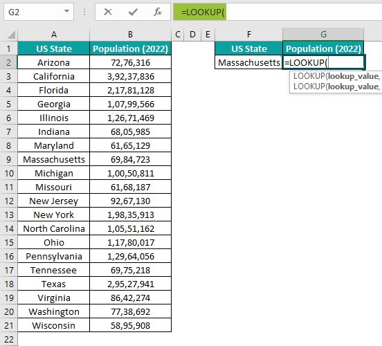
Next, enter the cell reference to the given lookup value, followed by a comma.
=LOOKUP(F2,

And then, enter the lookup_vector range, followed by a comma.
=LOOKUP(F2,A2:A21,
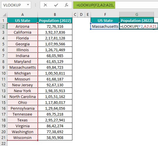
Next, enter the result_vector range, B2:B21.
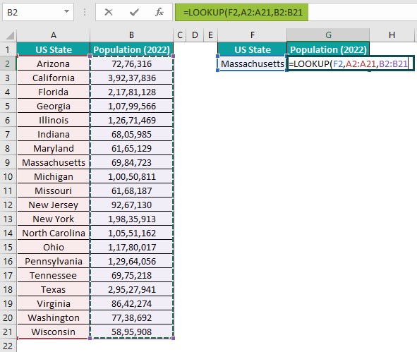
Finally, close the bracket.
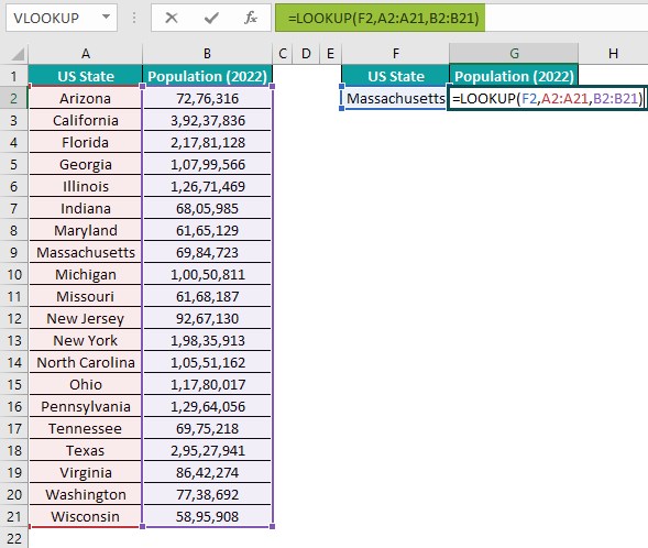
Step 3: Press Enter to achieve the required data in cell G2 of the lookup table.
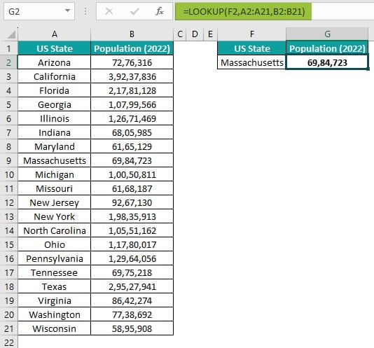
The LOOKUP function searches for the lookup value in the lookup_vector range A2:A21. And then, it returns the value from the same row of the result_vector range, B2:B21, as the lookup value.
Furthermore, if we change the lookup value in cell F2, as shown below:
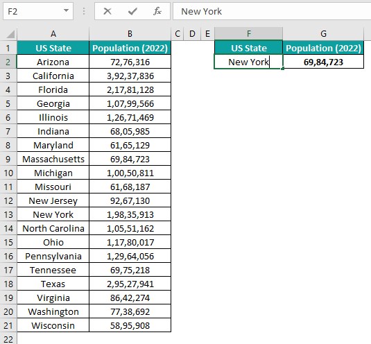
Then, pressing Enter will make the LOOKUP() in cell G2 automatically update the return value corresponding to the new lookup value.
#3 – Use INDEX + MATCH Function
The steps to build an Excel lookup table using the INDEX-MATCH function are as follows:
- Choose a cell range to show a lookup table.
- Enter the lookup table column headings.
- Enter the lookup value in the second cell of the lookup table’s first column.
- Choose the second cell in the second column as the target cell to display the output.
- Enter the appropriate INDEX-MATCH function in the target cell.
- Press Enter to obtain the required output in the lookup table.
Basic Example
The following table lists sales representatives at a firm and the sales they generated in July 2023.
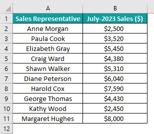
The task is to define an Excel lookup table in the cell range E1:F2 to look for a sales representative and determine their July 2023 sales figures.
Then, we can build the required lookup table in the target cell range using the INDEX-MATCH function.
Step 1: Choose cells E1 and F1, and update the column headings in the lookup table individually.
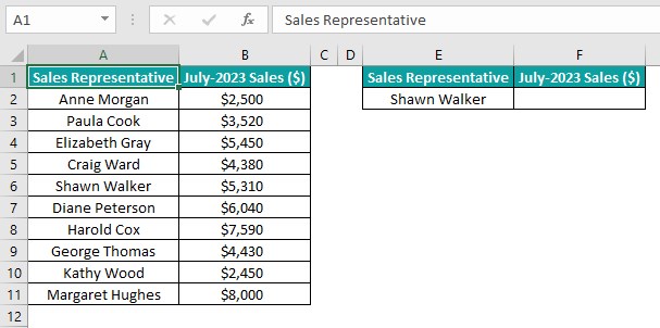
And then, select cell E2 and enter the required lookup value.
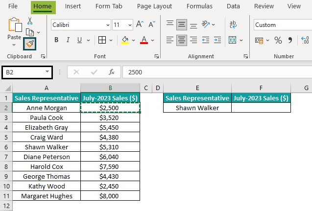
Step 2: First, we must set the correct data format in the target cell in the lookup table. And for that, select cell B2 and choose Home – Format Painter to copy the specific cell format.
And then, click cell F2 to apply the source cell data format.
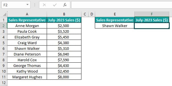
Step 3: Choose cell F2 and enter the Excel INDEX function.
=INDEX(

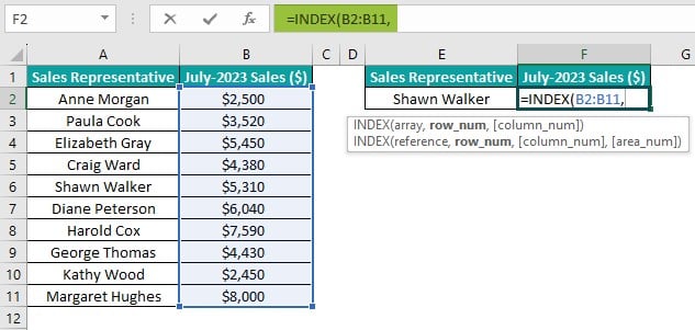
Next, enter the required array range, followed by a comma.
=INDEX(B2:B11,
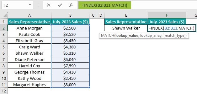
And then, enter the MATCH Excel function as the row_num argument value of the INDEX().
=INDEX(B2:B11,MATCH(
Next, enter the lookup value cell reference, followed by a comma.
=INDEX(B2:B11,MATCH(E2,

And then, enter the lookup array range, followed by a comma.
=INDEX(B2:B11,MATCH(E2,A2:A11,

Once we enter the comma, Excel will show the logical value options for the match_type argument. And as we want an exact match, we shall double-click the second option.
=INDEX(B2:B11,MATCH(E2,A2:A11,0

And then, enter to closing brackets to complete the formula.
=INDEX(B2:B11,MATCH(E2,A2:A11,0))
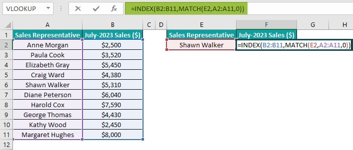
Step 4: Press Enter to obtain the required return value in the target cell F2 of the lookup table.

First, the MATCH() returns the position of the specified lookup value in the given range of A2:A11, 5. And then, the INDEX() returns the value in the cell at the intersection of column B range B2:B11 and row 5, which will be the cell B6 value.
Important Things To Note
- If we use the VLOOKUP() to define a lookup table in Excel. Then, we must ensure the source data is organized so that the function searches for the lookup value in the first column in the lookup range. And the column containing the return value should be on the right of the first column in the lookup range. Otherwise, the function will return an error value.
- The lookup_vector values should follow ascending order when using the LOOKUP(). Otherwise, the function output might be incorrect.

Frequently Asked Questions (FAQs)
We can do an Excel lookup table with IF statement using the following steps, explained with an example.
The table below lists products and their order quantity data.
Consider the requirement to build a lookup table in the cell range E1:F2, showing the order status of the specified product based on its order quantity data.
And the order status should be PROCEED if the order quantity equals or exceeds 5000. Otherwise, the order status should be DECLINE.
Then, the steps are as follows:
Step 1: Choose cells E1 and F1, and update the lookup table column headings individually.
Next, choose cell E2 and enter the required lookup value.
Step 2: Choose cell F2, enter the IF statement, and press Enter.
=IF(VLOOKUP(E2,A2:B11,2,0)>=5000,”PROCEED”,”DECLINE”)
First, the VLOOKUP() searches the lookup value in the specified range. And then, it returns the value in the same row of the cited column as the lookup value. Next, the IF() checks if the VLOOKUP() output equals or exceeds 5000.
In this case, the function returns the FALSE value as the IF condition does not hold.
Furthermore, we can change the lookup value in cell E2. And the IF statement in cell F2 of the lookup table will automatically update the corresponding output.

We can name a lookup table in Excel using the following steps:
1. Choose the lookup table range.
2. Select Formulas – Define Name to open the New Name window.
3. Update the required name in the Name field in the New Name window.
4. Click OK in the New Name window to close it and complete the lookup table naming action.
Alternatively, we can choose the lookup table range and enter the required name in the Name Box. The Name Box is on the left of the Insert Function box above the workspace. And then, press Enter to complete the lookup table naming action.
Excel lookup table from another workbook is possible. And the steps are as follows:
1. Open both workbooks. One workbook will be the active workbook, where we would have the lookup value and must display its corresponding return value. And the other one will contain the lookup range.
2. Choose a target cell in the active workbook and enter the VLOOKUP()
First, enter ‘=’, the function name, and an opening bracket.
And then, enter the lookup value or the cell reference to it, followed by a comma.
Next, go to the other workbook. Hover the mouse on the first cell of the first column in the lookup range. And with the mouse’s left key pressed, drag the mouse across the cell range to choose the required lookup range. Excel will show the chosen cell range, with the file name and sheet name in single quotes and an Exclamation Mark preceding it.
And then, enter a comma.
Next, enter the column number, followed by a comma. And then, enter the logical value indicating the required match type.
Finally, close the bracket.
3. Press Enter to execute the VLOOKUP(). The function will get executed in the target cell in the active workbook.
Download Template
This article must be helpful to understand the Lookup Table In Excel, with its formula and examples. You can download the template here to use it instantly.
Recommended Articles
This has been a guide to What Is Lookup Table In Excel. We learn to create it using VLOOKUP, LOOKUP, and INDEX plus MATCH functions with examples. You may learn more from the following articles –

Leave a Reply