
What Is Strikethrough In Google Sheets?
The Strikethrough in Google Sheets is a font feature, where a horizontal line, a dash or a cross is drawn in-between the selected cell value, indicating that it is stricken or no longer in use.
We use the Google Sheets Strikethrough instead of the Delete option, to show that the option or the text that was available,can be ignored or removed.
Use this Strikethrough In Google Sheets Template to follow along with the examples in this article.
Download Excel TemplateFor example, we have the data below of a string and let us apply the Strikethrough feature In Google Sheets and view the output.

Copy the cell value from cell A2 to B2 and click the STRIKETHROUGH option in Google Sheets on the cell B2 value, as shown below.

The output is shown above. We notice that the value does not change, but is untouched, and only a line appears as a strike in-between the text.
Key Takeaways
- The Strikethrough in Google Sheets is a feature that strikes through the words in the cells meaning, striking the text, numeric value or any other value from the center passed through the selected cell or a cell range.
- We can apply this feature for a cell value for just a letter, word or the entire cell value.
- All the methods used to apply the Strikethrough feature are the same methods used to remove them. Except in the Conditional Formatting method, we must delete the set rule, to remove the applied Strikethrough.
- The shortcut key to apply the Strikethrough is “Ctrl+Alt+5” keys, all pressed at once.
Top 4 Methods To Strikethrough In Google Sheets
The Top 4 Methods to Strikethrough In Google Sheets are as follows:
- Using Shortcut Key.
- Using Format Option.
- Using Quick Access Toolbar.
- Using Conditional Formatting.
Method #1 – Using Shortcut Key
The steps to apply the Strikethrough feature using Shortcut Key are,
Step 1: Choose the cell or cell range to apply Strikethrough.
Step 2: Click the shortcut keys “Alt+Shift+5”.
Method #2 – Using Format Option
The steps to apply the Strikethrough feature using Format Option are,
Step 1: Choose the cell or cell range to apply Strikethrough.
Step 2: Select the “Format” tab à click the “Text” option right-arrow à select the “Strikethrough” option, as shown below.

Method #3 – Using Quick Access Toolbar
The steps to apply the Strikethrough feature using Quick Access Toolbar are,
Step 1: Choose the cell or cell range to apply Strikethrough.
Step 2: Click the “Strikethrough (Alt+Shift+5)” option from the Quick Access Toolbar or also known as the Toolbar, below the Main Menu or Ribbon, as shown below.

Method #4 – Using Conditional Formatting
The steps to apply the Strikethrough feature using Conditional Formatting are,
Step 1: Choose the cell or cell range to apply Strikethrough.
Step 2: Select the “Format” tab – choose the “Conditional formatting” option. Then, we get the “Conditional format rules” window at the right, here, click the “Add another rule” option, as shown.

Step 3: Regardless of the default options, select the “Strikethrough” option and click “Done”, as shown below.
[Note: If required we can also set a rule for multiple cells or a cell range and apply the “Strikethrough” option.]

How To Remove Strikethrough In Google Sheets?
We can Remove Strikethrough in Google Sheets using the same methods used to Add them, namely,
- Using Shortcut Key.
- Using Format Option.
- Using Quick Access Toolbar.
Method #1 – Using Shortcut Key
The steps to remove the Strikethrough feature using Shortcut Key are,
Step 1: Choose the cell or cell range where the Strikethrough feature is already applied.
Step 2: Click the shortcut keys “Alt+Shift+5”.
Method #2 – Using Format Option
The steps to remove the Strikethrough feature using Format Option are,
Step 1: Choose the cell or cell range where the Strikethrough feature is already applied.
Step 2: Select the “Format” tab – click the “Text” option right-arrow – select the “Strikethrough” option, as shown below.

Method #3 – Using Quick Access Toolbar
The steps to remove the Strikethrough feature using Quich Access Toolbar are,
Step 1: Choose the cell or cell range where the Strikethrough feature is already applied.
Step 2: Click the “Strikethrough (Alt+Shift+5)” option from the Quick Access Toolbar or also known as the Toolbar, below the Main Menu or Ribbon, as shown below.

Examples
Let us consider some specific Strikethrough in Google Sheets examples using the top 4 methods we just learnt.
Example #1 – Using Shortcut Key
The dataset given below consists of random data and we will apply Strikethrough using the Shortcut Keys. We have copy pasted the original data in the result cells too.

The procedure to apply Strikethrough using the Shortcut Keys is,
Select cells B2 to B7 and press the shortcut keys “Alt+Shift+5”, to get the following Strikethrough results.

Example #2 – Using Format Option
The dataset given below consists of a few company names and we will apply Strikethrough using the Format Option. We have copy pasted the original data in the result cells too.

The procedure to apply Strikethrough using the Format Option is,
Choose the cells B2 to B11 – select the “Format” tab – click the “Text” option right-arrow – select the “Strikethrough” option, as shown below.

We will get the following output.

Example #3 – Uisng Quick Access Toolbar
The dataset given below consists of famous actors and actresses’ names and we will apply Strikethrough using the Quick Access Toolbar. We have copy pasted the original data in the result cells too.

The procedure to apply Strikethrough using the Quick Access Toolbar is,
Select cells B2 to B7 and click the “Strikethrough (Alt+Shift+5)” option from the Quick Access Toolbar, as shown below.

We get the following output.

Example #4 – Using Conditional Formatting
The dataset given below consists of normal conversational questions and we will apply Strikethrough using the Conditional Formatting. We have copy pasted the original data in the result cells too.

The steps to apply the Strikethrough using Conditional Formatting are,
Step 1: Choose the cells B2 to B6 – Select the “Format” tab – choose the “Conditional formatting” option. Then, we get the “Conditional format rules” window at the right, here, click the “Add another rule” option, as shown.

Step 2: Select the “Single color” tab and under the “Format rules” section,
- First, choose the “Text contains” option from the “Format rules if…” option drop-down and type “how”, in the field that appears below.
- Next, click the “Strikethrough” option form the “Formatting style” options and select the desired color, here, cyan.
- Finally, click the “Done” option, as shown below.

We will get the following output, i.e., if the selected text has the word “how”, then, the Strikethrough is applied to the selected data.

Important Things To Note
- We can apply the Strikethrough in Google Sheets, even to just an alphabet, a word, entire cell value or a cell range. For example,
MyName isJohn orMy Name is John. - When we apply Strikethrough in Google Sheets to any cell, the cell’s value does not change, and only the horizontal line appears. So, for example, “
TEXT” and “TEXT” are equal. - We can apply Strikethrough in Google Sheets by creating a “New Rule” using “Conditional Formatting”.
Frequently Asked Questions (FAQs)
An alternate method to apply Strikethrough in Google Sheets is by using the “Paint format” tool.
For example, we have a cell value where the Strikethrough feature is already applied, as shown below.
Suppose, in cell D1 we have a cell value that needs to have Strikethrough applied, then, select cell A2 and clickthe “Paint format” option to copy the format, as shown below.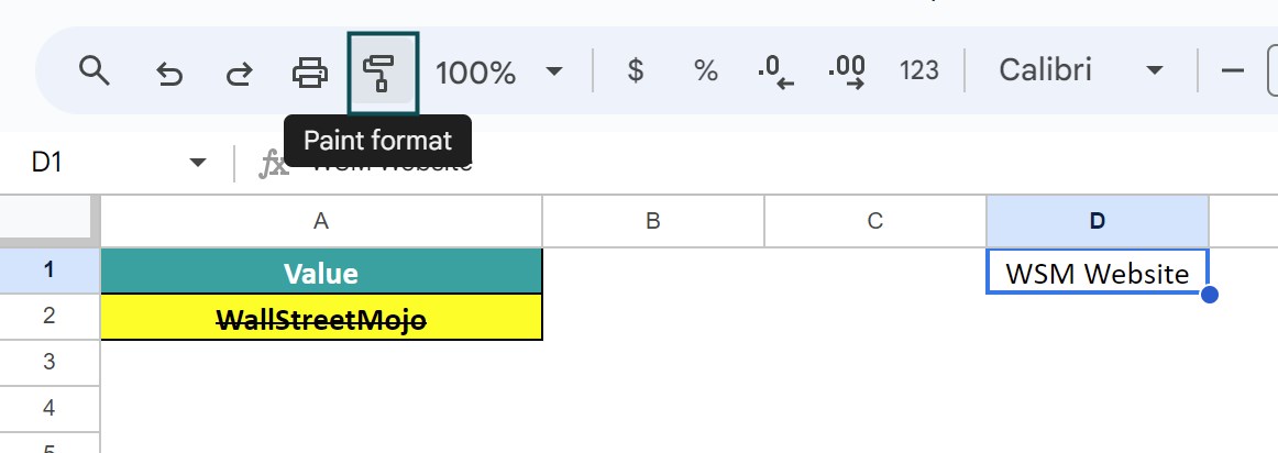
Now, paste it on cell D1 and automatically the entire formatting of the copied cell will appear on the pasted cell, as shown below.
We notice that the “Paint format” or the “Format Painter” copy-pasted the entire formatting such as Bold font and the yellow color fill, along with the Strikethrough.
Yes, we can use the copy-paste method toapply Strikethrough in Google Sheets as follows:
For example, we have a cell value where the Strikethrough feature is already applied, as shown below.
Suppose in cell A5 we have a cell value that needs to have Strikethrough applied, then, right-click on cell A2, clickthe “Copy” option, as shown below.
Finally, right-click on cell A5, click the “Paste special” option right-arrow and select the “Format only” option, as shown below.
We will get the following output.
A few reasons the Strikethrough in Google Sheets may not work is because,
• We did not copy the existing Strikethrough cell value to paste on the other cell value.
• Instead of the “Copy à Paste Special – Format” option, we used the normal “Copy – Paste” option. And so, the value is pasted and not the format, as we saw in FAQ2.
• The shortcut keys were incorrectly used.
• The conditional formatting was selected for a cell and not a cell range or the rule set was incorrect.
Use this Strikethrough In Google Sheets Template to follow along with the examples in this article.
Download Excel TemplateRecommended Articles
Continue with these related resources when you want the next practical step in this topic.
- Columns In Google Sheets
- Add Column In Google Sheets
- Insert Rows In Google Sheets
- AutoFit In Google Sheets
- Border In Google Sheets
Explore the full Google Sheets Basics guide or browse Google Sheets Resources.