
What is SUMPRODUCT in Google Sheets?
SUMPRODUCT in Google Sheets finds the product of the corresponding values in the given arrays and returns its sum. Thus, it can help perform advanced calculations and compare numbers in two or more ranges. Therefore, if you need to find both the product and the sum of arrays or corresponding ranges, you can use the SUMPRODUCT. Thus, you can compute the aggregated number of products, especially when checking product sales.
For instance, a salesman sells some items in a shop and needs to keep track of the total sales he made. He can use the SUMPRODUCT function to calculate it. To find the total sales made, one must multiply the price of each item by the number of items sold and get the sum. To find the sales amount, we use the following formula: =SUMPRODUCT(A2:A5, B2:B5) in cell B6.

Use this SUMPRODUCT in Google Sheets Template to follow along with the examples in this article.
Download Excel TemplateKey Takeaways
- The SUMPRODUCT function in Google Sheets multiplies the corresponding values in two or more ranges and then sums their result.
- Its syntax is as follows: =SUMPRODUCT(array1, [array2, …]), where each array is a range or set of values you want to multiply and sum.
- All ranges we use in the formula must contain the same dimensions (same number of rows and columns), or we get an error.
- SUMPRODUCT can be combined with conditions, such as logical tests (A2:A10=”John”), to perform filtered calculations without the need for any extra helper columns.
- It is useful for calculating values like weighted averages, making it a versatile tool for data analysis.
Syntax
SUMPRODUCT in Google Sheets is a handy tool that multiplies matching items in two or more lists and then adds them up in one go. The usefulness of this function can be seen in the succeeding examples below. Before that, let us look at the SUMPRODUCT in Google Sheets formula below.
=SUMPRODUCT(array1, [array2, …])
- array1 – The first array or range whose entries will be multiplied with corresponding entries in the second such array or range.
- array2, … – [ OPTIONAL – {1,1,1,…} with same length as array1 by default ] – The second array or range whose entries will be multiplied with corresponding entries in the first such array or range.
How To Use SUMPRODUCT Function in Google Sheets?
SUMPRODUCT in Google Sheets is an extremely versatile formula that can handle data in different arrays in an elegant way by comparing and summing them. We can use the SUMPRODUCT function in two ways.
- Can be entered manually in a cell
- Access from the menu bar.
Entering SUMPRODUCT in Google Sheets Manually
To gain a detailed understanding of how SUMPRODUCT works by entering it manually, consider the following example. We have the grades of a student and their weightage. Let us calculate the total marks of the student. This can be done by multiplying the weightage by each score and finally summing them up.
Step 1: Enter all the details in a table, as shown below.

Step 2: Next, enter the following formula in an empty cell:
First type =, followed by the function name. Open the parentheses, enter the two ranges separated by a comma. Close the parentheses and press Enter.
=SUMPRODUCT(A2:A5,B2:B5).

Step 3: You can find the total score secured by the student.

That’s how easy performing the multiple calculations of product and sum using SUMPRODUCT is.
Entering SUMPRODUCT Through the Menu Bar
Besides manually entering the formula, you can also use the SUMPRODUCT function by entering it through the main menu.
- Place the cursor where you want the formula to be entered.
- Go to Insert → Function → Math.
- From the list, choose SUMPRODUCT.
- In the formula bar, enter the ranges you want multiplied and summed (e.g., A2:A5, B2:B5).
- Press Enter to get the result.
Examples
We use SUMPRODUCT to calculate the sum of the products of the corresponding entries in two ranges of equal size. This can be used in a wide variety of applications, as shown in the example below.
Example #1
We have some sales details of some employees in a store. The owner wished to calculate the individual sales amount of each salesperson. Let us look at how easily he can calculate it using the SUMPRODUCT formula.
Step 1: Enter the details in a Google Sheets as shown below.
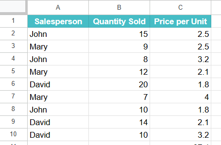
Step 2: The total sales of a particular employee can be obtained by entering the following formula in cell C11.
=SUMPRODUCT((B2:B10*C2:C10)*(A2:A10=”David”))

- Here, we take the values in Column B, the quantity sold, and multiply it with the price per unit in Column C to find the sales details.
- Using the conditional operator “=”, we can find the commission received by a particular employee.
- We the find these sales details of the employee called “David.”
Step 3: Press Enter. Thus, the SUMPRODUCT function can find the sum and product of specific values in a range for a particular entity.

You can also use SUMPRODUCT with a search criteria of multiple conditions using SUMPRODUCT. For example,
=SUMPRODUCT((A2:A10=”Science”)*(B2:B10=”Emma”))
gives you the marks secured by the student Emma in Science over a whole year if you have a table containing marks of different students in various subjects throughout the year.
Example #2 – Using SUMPRODUCT with a Condition
A store owner wishes to calculate the total sales value of all the high-priced products, priced above $3. For this he decides to use SUMPRODUCT instead of filtering the data manually. Let us look at how we can use SUMPRODUCT with a condition.
Step 1: Enter the details in a sheet, as shown below:

Step 2: We can use the following function.
=SUMPRODUCT((C2:C7>3)*(B2:B7)*(C2:C7))

Here it means,
- (C2:C7>3) → checks which prices are above $3
- (B2:B7) → quantity sold.
- (C2:C7) → price per unit.
SUMPRODUCT multiplies them and adds them up for those products that cost less than $3.

Example #3 – Using SUMPRODUCT with IF Function
A company wants to calculate bonus payouts for its employees if their sales exceed $400. The bonus is 10% of their total sales. Let us use the SUMPRODUCT function for this very purpose and see how it can be done easily.
Step 1: Let us enter all the details in a Google Sheet.

Step 2: Click on the cell where you want the total bonus payout to appear. Enter the formula as shown below:
=SUMPRODUCT(IF(B2:B6>400, B2:B6*C2:C6, 0))

Explanation:
- IF(B2:B6>400, …) → checks if sales exceed $400.
- B2:B6*C2:C6 → calculates the bonus for qualifying employees.
- If sales don’t exceed $400, it returns 0 for that row.
- SUMPRODUCT adds up all the calculated bonuses.
Step 3: Press Enter. The formula returns the total bonus payout for employees who meet the sales condition.

This is a very useful method when performing conditional calculations where you only want to include certain rows in your totals.
Important Things to Note
- In SUMPRODUCT, the array arguments should have the same dimensions to avoid the #VALUE! Error. If we use the formula =SUMPRODUCT(A2:A7, B1:B3), we get a #VALUE error since the ranges aren’t the same size.
- SUMPRODUCT does not support the use of wildcard characters.
- SUMPRODUCT treats non-numeric array entries as zeros.
Frequently Asked Questions (FAQs)
One of the best uses of SUMPRODUCT in Google Sheets is the easy method with which one can find the weighted average. One can use it to calculate the weighted average where each value is assigned a particular weight. The formula we use to find the weighted average is as shown below:
=SUMPRODUCT(values, weights) / SUM(weights)
Let us consider an example. The values are contained in the range A2:A6, and their corresponding weights are in cell B2:B6. We calculate the weighted average using the formula shown below:
=SUMPRODUCT(A2:A6,B2:B6)/SUM(B2:B6).
Text values cannot be used directly in the multiplication and addition part. However, we can use text to check certain conditions, as we did in Example 1 above, where we used the condition (A2:A10=”David”), to only include those rows where the text matches. This method of using text to filter calculations by category or name is very helpful.
SUMPRODUCT is very versatile in that we can use it even with multiple criteria.
For instance, we can use a formula like
=SUMPRODUCT((A2:A10<B2:B10)(C2:C10=”Peter”)).
Here, we use Asterisk () as the AND operator. It checks how many times the number of real sales (column A) was less than planned sales (column B) for the salesman named Peter.
We use SUM when we just need to add up all the values of the numbers or range supplied, for instance, =SUM(A1:A5). SUMPRODUCT first multiplies matching values from the different ranges before summing them. Thus, SUMPRODUCT is ideal in scenarios such as calculating the total sales (quantity × price) or weighted averages in a single step.
Use this SUMPRODUCT in Google Sheets Template to follow along with the examples in this article.
Download Excel Template