
What Is VLOOKUP Table Array In Google Sheets?
The VLOOKUP Table Array in Google Sheets is the second argument in the VLOOKUP function, a data range containing a minimum of two columns. The first column is to find the lookup value and a column on the right of the first column, within the chosen data range, will contain the value we require the VLOOKUP() to return in the target cell.
Users can specify the table array in the VLOOKUP() as a relative or absolute reference to a dataset in the same or different sheet. Thus, it makes the VLOOKUP function resourceful for fetching the corresponding data from within and outside the current sheet.
For example, the first table lists items, their categories and quantities. We will update the category for the item cited, here, Oranges, in the second table based on the first table data.
Use this VLOOKUP Table Array In Google Sheets Template to follow along with the examples in this article.
Download Excel Template
Therefore, select cell F2, enter the formula =VLOOKUP(E2,A2:B7,2,0) and press “Enter”.

The output is shown above as Fruit. The second argument in the VLOOKUP() is the table array and is a relative reference to the cell range A2:B7. It implies that the function in the target cell searches the lookup value, Oranges, in the cell range A2:B7, in the first column, of the specified table array. Once it locates the first occurrence of the lookup value in column A, cell A5, it returns the data in the same row of the last column of the given table array, cell B5 value, as Fruit.
Key Takeaways
- The VLOOKUP table array in Google Sheets is the data range, with a minimum of two columns, which we supply as the second argument value to the function.
- Users can supply the appropriate table array to the VLOOKUP() when they must fill one table based on the data provided in another table in the same or different worksheet.
- We can supply the table_array argument value to the VLOOKUP() as a relative or absolute reference to a cell range in the same or different sheet. We can also keep it variable using the INDIRECT() function using the named range method.
Syntax
The syntax of the VLOOKUP formula in Google Sheets is,

The arguments of the VLOOKUP formula in Google Sheets are,
- search_key – The value to lookup or search in the very first column of the cell range.
- range – The dataset, table array or the cell range where we find the search_key.
- index – It is always a number, which specifies the column number of the dataset or cell range that contains the return value.
- [is_sorted] à It returns the exact or approximate value based on the selection as,
- If we select “0” [False], it will return the exact match or else return an error.
- If we select “1” [True], then it will give an approximate match.
How To Use VLOOKUP Table Array In Google Sheets?
We can use the VLOOKUP Table Array Google Sheets Function in 2 ways, namely,
- Access from the toolbar.
- Enter in the worksheet manually.
#1 – Method – Access from the toolbar –
Choose an empty cell for output à select the “Insert” tab à click the “Function” option right arrow à click the “Lookup” option right arrow à select the “VLOOKUP” function, as shown below.

The VLOOKUP formula appears as shown below.

Select the argument values as cell references or cell rangeand press “Enter”.
#2 – Enter in the worksheet manually
- Select an empty cell to display the output.
- Type =VLOOKUP( in the chosen cell. [Alternatively, enter =V or =VL and click the VLOOKUP function from the suggestions Google Sheets lists.]
- Enter the cell values or references as the argument values.
- Close the brackets and press Enter to obtain the logical results in the target cells.
Examples
Let us consider some examples of Google Sheets VLOOKUP table array and learn how to provide the table array value to the VLOOKUP() to use the function effectively.
Example #1
We have the data given below, where the first table lists employees, their designations and joining dates. Let us find the joining date of the employee, here, Tabitha, by giving a defined name to the table array or the cell range.

The steps to find the required data using VLOOKUP and the name range are as follows:
Step 1: Let us first create the named range.
First, select the “Data” tab à click the “Named ranges” option, as shown below.

Next, the “Named ranges” window appears on the right side. Here, click the “Add a range” option, as shown below.

The following window appears below.

Finally, enter the name “Emp_Data” in the first field, enter or select the cell range, A1:C7, in the second field and click “Done”, as shown below.

We can see the named range, i.e., Emp_Data, created as shown below.

Step 2: To find the required employee’s date of joining, select cell B10, enter the formula =VLOOKUP(A10,emp . Immediately we see the created named range, as shown below.

Step 3: Select the named range, complete the formula, and press “Enter”, as shown below.
The complete formula is =VLOOKUP(A10,Emp_Data,3,0).

The output is shown above as 4/10/2024.
- We created the source dataset as a named range, Emp_Data which enables the function to search for the lookup value, Tabitha, in the first column of the source data.
- The argument index value is 3. It implies that the function must return the required value from the third column, column C, counted from the first column in the specified table array.
- So, once the function finds its first occurrence in the first column, cell A4, it returns the data in the same row of the column specified by col_index_num, cell C4 value, 4/10/2024.
Example #2
We will use the INDIRECT Google Sheets function as the table_array in the VLOOKUP() to look up the same value from multiple tables given below that contains a list of students, their scores and their ranks in Mathematics and Science tests and find the ranks of Mandy in the two tests.

The steps to use an INDIRECT()-based variable table array in the VLOOKUP() are as follows:
Step 1: First, create another table for the output cells, E1:H3, as shown below.

Step 2:
- Select cell H2, enter the VLOOKUP() containing the INDIRECT() formula =VLOOKUP(E2,INDIRECT(F2),3,0) and press Enter.

- Select cell H3, enter the VLOOKUP() containing the INDIRECT() formula =VLOOKUP(E3,INDIRECT(F3),3,0) and press Enter.

The output is shown above as Rank 1 in Mathematics and Rank 4 in Science for Mandy. We can see the highlighted values for our reference, as shown below.

Example #3
Let us see a VLOOKUP table array different sheet example.
We have two worksheets, SalesRep_Sales_Commission and Sales_CommissionPercentage as shown below.
- The first one contains a list of sales representatives at a firm and their achieved sales targets.

- The second sheet contains the commissions one can earn for different sales figures.

And we must update the commission the sales representatives earned for their achieved sales targets in column C of the first sheet based on the second worksheet data.
Therefore, applying the VLOOKUP table array different sheet method, with an approximate match, will help us update the required values in the target cells. However, ensure the data in the first column in the table array, referenced from the second sheet, must be in ascending order. Otherwise, the VLOOKUP() may return an incorrect value based on an approximate match.
The steps to calculate the commission percentage are as follows:
Step 1: Select the cell C2, enter the formula =VLOOKUP(B2,Sales_CommissionPercentage!A1:B6,2,1), as shown below.

Step 2: Press “Enter” and drag the formula from cell C2 to C7 using the fill handle, as shown below.

We get the output shown above with a message to make the cell range selected absolute or to lock the cells. Otherwise, we get the “#NA” error, as seen in cell C7. Therefore, click the tick mark.
Then. the formula becomes =VLOOKUP(B2,Sales_CommissionPercentage!$A$1:$B$6,2,1) and the output is shown below.

Let us see the cell C2 formula to understand how the table array reference from another sheet works.
The VLOOKUP() searches for the lookup value in cell B2 of the first sheet, $19000 and in the cell range A2:B6 in the second worksheet. As the lookup value is over $15,000 and we chose the last argument value as TRUE, the VLOOKUP() finds an approximate match in cell B4. Thus, it returns the commission percentage in the same row in column C, the cell B4 value, 6.00%, as the output.
Important Things To Note
- Ensure the number of columns in the VLOOKUP table array equals at least the number supplied as the index argument value.
- To use the VLOOKUP() in continuous cells, with the table array range being the same, lock the table array when supplying it to the VLOOKUP() in the first cell.
- If the first column in the table array does not contain the lookup value or the lookup value is below the lowest value in the first column in the lookup range, then, the VLOOKUP() may not work for the specified table array.
Frequently Asked Questions (FAQs)
We can lock the table array in the VLOOKUP function by using the following methods:
• Absolute referencing the cell range when supplying it as the table_array argument value to the VLOOKUP().
• Supplying a named range as the table_array argument value to the VLOOKUP().
• Updating the VLOOKUP() in the worksheet and password-protecting the sheet.
A few reasons the VLOOKUP table array in Google Sheets may not work are,
1) The first column of the specified table array does not contain the lookup value.
2) he cell format for currency, percentage, etc, is not applied to the result or target cells.
3) The table array or cell ranges are not locked or not made absolute, hence, we get “#NA” or “#REF” errors.
4) The lookup value is below the least value in the table array’s first column.
We often cannot remember in which category the “VLOOKUP” function falls. Then, we can insert the function as follows:
Choose an empty cell – select the “Insert” tab – click the “Function” option right arrow – click the “All” option right arrow – select the “VLOOKUP” function, as shown below.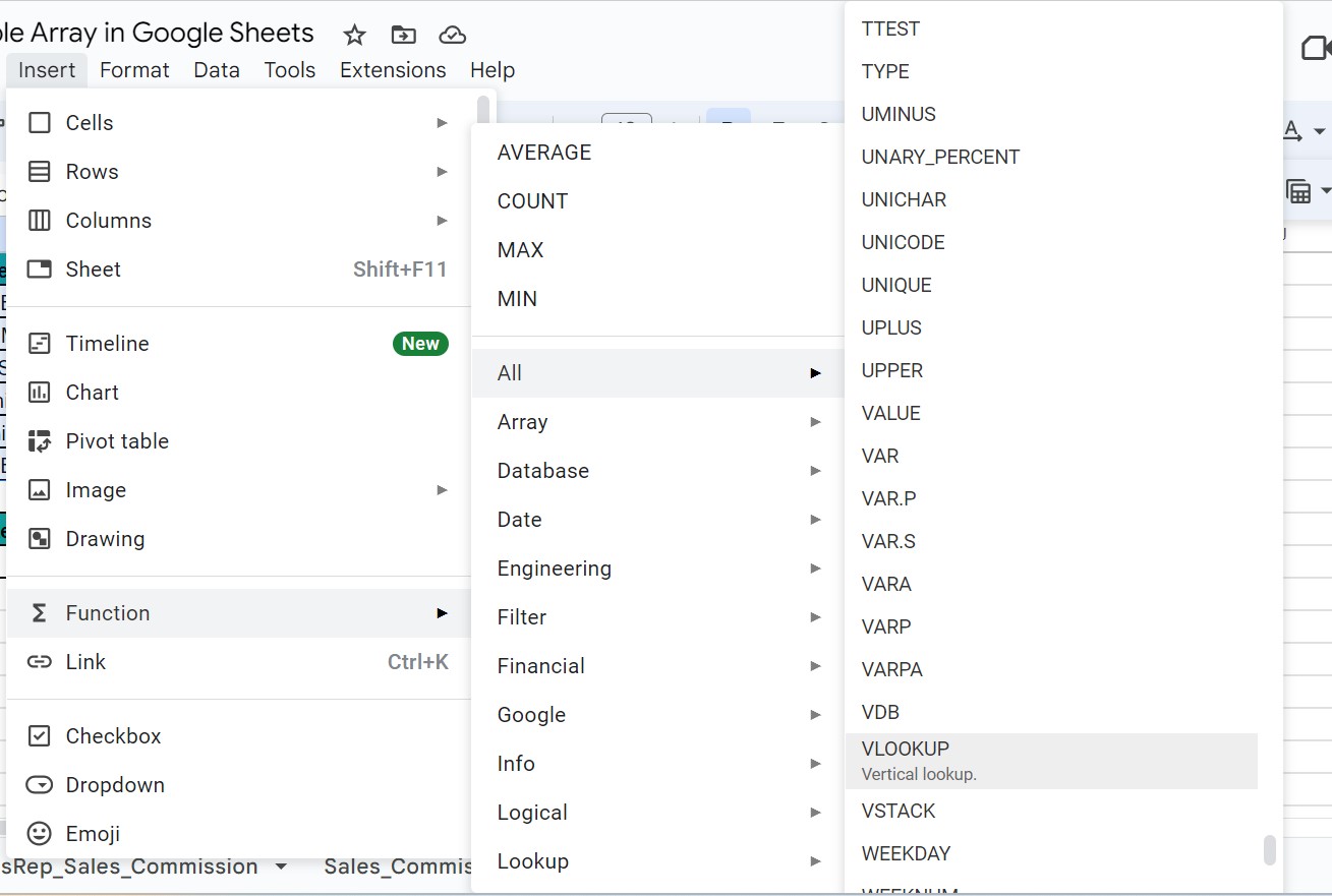
However, as always, entering the function manually, is the best way to avoid confusion.
Alternatively, we can also find the Function icon to insert the VLOOKUP function by following the path shown below.
• Choose an empty cell – click the “More” option represented by the three vertical dots at the end of the toolbar, as shown below.
• A list of icons appears when we click the “More” option. Here, click the “Functions” icon, as shown below.
• When we click the “Functions” icon, we get the details shown in the below image.
From here, we know the rest to select the required function.
Use this VLOOKUP Table Array In Google Sheets Template to follow along with the examples in this article.
Download Excel TemplateRecommended Articles
Continue with these related resources when you want the next practical step in this topic.
- LOOKUP in Google Sheets
- HLOOKUP In Google Sheets
- VLOOKUP True In Google Sheets
- INDEX MATCH Function In Google Sheets
- MATCH Function In Google Sheets
Explore the full Google Sheets Lookup Functions guide or browse Google Sheets Resources.