What Do You Mean By Excel Dynamic Named Range?
The dynamic named range in Excel enables one to build a named range that automatically adjusts its size to accommodate the changes made to the data. So, one can develop formulas referencing cell ranges that one does not have to update manually whenever the supplied data gets updated.
Users can use the dynamic named range in Excel feature for developing charts and Pivot Tables.
For example, the table below shows a list of experiments and their results.
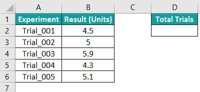
And the task is to count the total number of trials in column A, with the list being dynamic. Assume the target cell is D2.
Then, we can make a dynamic named range in Excel using column A in the OFFSET and COUNTA functions-based formula in the Define Name feature in the Formulas tab.
Finally, we can use the COUNTA(), with the dynamic named range as the input, in the target cell to obtain the total trials count, which changes every time we modify the source list.
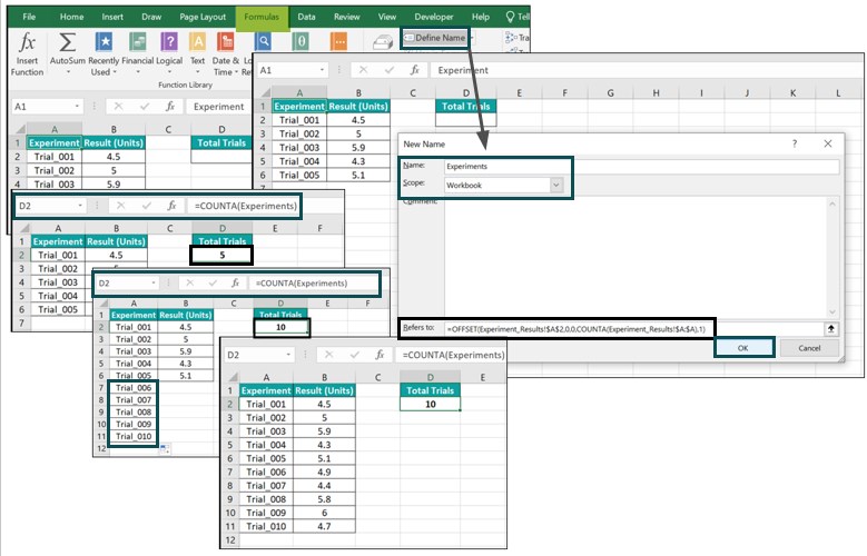
In the above example, we use the Define Name option in the Formulas to open the New Name window. And then, we enter a valid name and set the scope for the required range in the first two fields in the window.
Next, we enter the formula based on the OFFSET() containing the COUNTA() in the fourth field and click OK to make a dynamic named range in Excel, Experiments.
And then, we enter the Excel COUNTA function in the target cell D2, with the argument value being the defined name, Experiments.
Initially, column A shows five trials. So, the COUNTA() output is 5. But, once we add five more trials in column A, the COUNTA() input updates automatically and returns the value of 10. And then, we can update the trial results for the new entries to complete the table.
Thus, the dynamic named range using OFFSET in Excel simplifies the formula and reduces the possibility of errors.
Table of contents
Key Takeaways
- The dynamic named range in Excel option enables one to create variable-sized named ranges that adjust by changing height and width based on the count of non-empty cells.
- Users can use the Excel dynamic named range option to create dynamic pivot tables and plots.
- We can use the OFFSET or INDEX function with the COUNTA function in the Define Name feature to create a dynamic named range.
- We can use the dynamic named range option with the Data Validation feature for practical results.
How To Create Excel Dynamic Named Range?
The steps to create the dynamic named range in Excel are as follows:
- Create a list of the required data in a worksheet.
- Select the Formulas tab – Define Name – Define Name to open the New Name window. [Alternatively, we can press Alt + M + M + D to access the New Name window. Otherwise, use Ctrl + F3 to access the Excel Name Manager window and select the New option to open the New Name window.]
- Enter the name we want to use for the dynamic range based on the existing list in the Name field. Next, enter the scope using the Scope field drop-down list. And then, enter the following Excel OFFSET function or Excel INDEX function containing the COUNTA() in the Refers to field.
=OFFSET(first_datacell,0,0,COUNTA(column),1)
Or
=first_datacell:INDEX(column,COUNTA(column)) - Finally, click OK.
Rules For Creating Dynamic Named Range In Excel
The following rules will ensure we create a valid dynamic named range in Excel:
- The name is not case-sensitive and can be up to 255 characters.
- The name must start with a letter, the Underscore (‘_’) or a Backslash (‘\’).
- The name must not contain any spaces.
- The name cannot be a cell reference.
- The name cannot be “c”, “C”, “r”, or “R” since Excel utilizes them as selection shortcuts.
Examples
The following examples explain how to create and effectively use the dynamic named range in Excel option.
Example #1
We shall see an example of a dynamic named range using OFFSET in Excel.
The table below lists smartphones and the total ordered units of each smartphone.

Consider the source dataset is dynamic, with the columns A and B data editable and data added and removed from the lists according to the requirements.
And the task is to calculate the total smartphone units ordered based on the dynamic source data. Assume the target cell is E1.
Then we can first create a dynamic named range with the column B cells using the Define Name option with the OFFSET().
And then, use the dynamic named range as the input in the Excel SUM function in the target cell to achieve the required output.
Step 1: Choose Formulas – Define Name.

Step 2: The New Name window will open, where we must enter a valid name for the named range in the Name field, Total_Smartphones_Ordered.
Next, let the Scope be the default value, Workbook.
And then, enter the following OFFSET() in the Refers to field to make the named range dynamic.
=OFFSET(Smartphone_Orders!$B$2,0,0,COUNTA(Smartphone_Orders!$B:$B),1)

The OFFSET() syntax is:

In the current scenario:
- reference: The first item we want to include in the named range. It is the cell B2 value. And clicking cell B2 to enter it in the OFFSET() in the Refers to field will display it automatically as an absolute cell reference with the sheet name. And if it is not a cell or range, the function output will be the #VALUE! error in Excel.
- rows, cols: As we do not have to offset any columns or rows, the two argument values are 0.
- height: The Excel absolute reference to the required column in the COUNTA() to obtain the count of non-blank cells in the specified column. It will give the total rows we want as the returned reference. In this case, it is column B. So, clicking the column B header will select the entire column, displaying its absolute reference with the sheet name.
- width: It is one since we want only one column as the returned reference.
Step 3: Click OK.
Step 4: Choose cell E1 and enter the SUM().
=SUM(
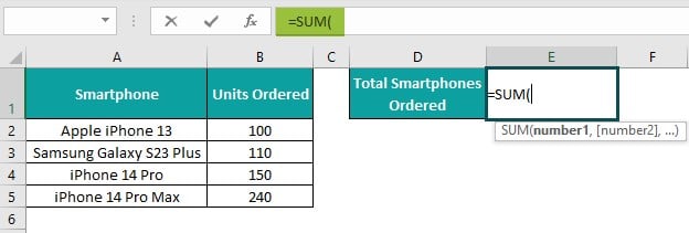
Next, we must enter the dynamic named range containing the ordered smartphone units data. And for that, type “to” inside the SUM().
Excel will list the functions and defined names starting with the specified phrase. Double-click on the required defined name, Total_Smartphones_Ordered, to select it.

=SUM(Total_Smartphones_Ordered

And then close the bracket to obtain the following formula:
=SUM(Total_Smartphones_Ordered)

Step 5: Press Enter to view the SUM() output in the target cell E1, 600.

The output is the sum of the ordered units of each smartphone in the cell range B2:B5.
Next, let us add more smartphone models in the cell range A6:A9.
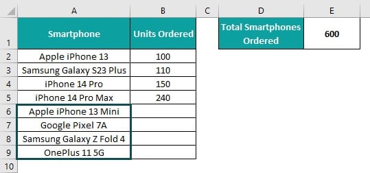
And then, updating cells B6 to B9 with the units ordered data for the newly appended smartphone models will automatically change the SUM() output.
It is because we defined column B as a dynamic named range and supplied it as the SUM() argument value. And the function output changes with every update we make in the dynamic named range, be it existing value changes or adding or removing data.


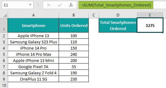
Thus, the OFFSET() returns a variable-sized range that expands and shrinks by modifying the height and width, considering the count of non-empty cells.
Example #2
We shall see an example of Excel dynamic named range with INDEX and COUNTA functions.
The table below shows students’ test scores and their aggregates.
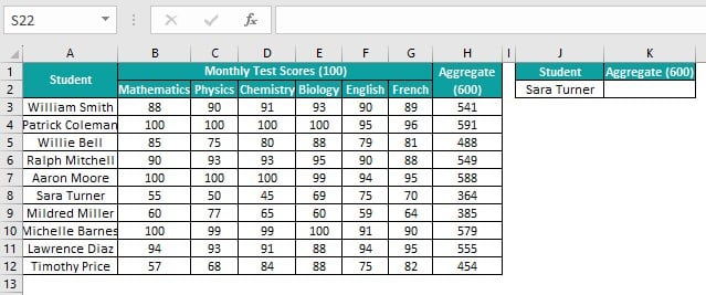
The given dataset is dynamic, with the current data editable, and we can add or remove data.
And the requirement is to update the aggregate of the student specified in cell J2 in the target cell K2.
Then, we can create an Excel dynamic named range with INDEX and COUNTA functions for the lookup and return ranges. And then use them in the INDEX-MATCH function in the target cell to achieve the required output.
Step 1: Select Formulas – Define Name to access the New Name window.

Step 2: Enter the required valid name for the named range in the Name field, Students, in the New Name window. And let the Scope be the default value, Workbook.
And then, enter the following INDEX() in the Refers to field to make the named range dynamic.
=Students_Aggregate!$A$3:INDEX(Students_Aggregate!$A:$A,COUNTA(Students_Aggregate!$A:$A))

Clicking OK in the New Name window will create the dynamic named range for the lookup range.
Step 3: Iterate steps 1 and 2 to create the dynamic named range for the return range.

However, we must enter a new valid name in the Name field in the New Name window, Student_Aggregate. And use the following formula in the Refers to field.
=Students_Aggregate!$H$3:INDEX(Students_Aggregate!$H:$H,COUNTA(Students_Aggregate!$H:$H))

And click OK to exit the New Name window.
Here is how to interpret the above formulas. Each expression contains two parts, separated by a Colon (the range or reference operator).
The first part, before the Colon, is the absolute reference to the first cell in the required column.
And the second part, which is after the Colon, includes the INDEX() to determine the ending reference.
The INDEX() syntax is:

In the above scenario, we shall consider the first syntax.
- array: The entire column A and column H will be the array range in each case. And clicking the columns A and H headers will show them automatically as an absolute reference with the sheet names in the respective formulas.
- row_num: It is the COUNTA() with columns A and H as the input in each case since we require the count of non-blank cells in each column.
Thus, the formula deduces to a cell reference, reference operator, and INDEX() output.
Ideally, the INDEX() output will be a value. But, since we use the reference operator, the Colon, the function output is a reference, $A$12and $H$12, in each case.
And hence the two resulting defined name ranges are $A$3: $A$12 and $H$3: $H$12.
Step 4: Choose cell K2 and enter the INDEX().
=INDEX(
Next, we must enter the return range as the first argument value. So, for that, type “Stu” for Excel to list all the functions and named ranges starting with the specified phrase.
And as the Student_Aggregate is the return range, double-click it to choose it.

Next, enter a comma.

And then, enter the Excel MATCH function, with the first argument value being the lookup value’s cell reference, J2, followed by a comma.

Next, the lookup_array will be the dynamic named range, Students. So, enter “stu” for Excel to list the functions and named ranges starting with the cited phrase. Double-click Students to select it, followed by a comma.

Next, Excel will list the options to decide the match type. Double-click on the 0 option for an exact match.


Finally, close the parentheses.

Step 5: Press Enter to view the INDEX() output in the target cell K2.

Next, assume we add new data to the existing source dataset.

And once we update cell J2 with a new lookup value from the newly-appended data, the INDEX() output in cell K2 automatically updates to give the required output.

Please note that entering only the absolute references in the Refers to field in the New Name window will work when the cell or range references are in the current worksheet. However, when the cell or range references are not in the current sheet, we must enter the concerned sheet name, followed by the Exclamation Mark, before the absolute reference.
And the above point applies to both methods, explained in the Examples section.
Important Things To Note
- The dynamic named range in Excel will work only when we follow the naming convention and rules for defining the names of the required ranges.
- Ensure the reference argument in the OFFSET() is a cell or range reference to avoid the function returning the #VALUE! error.
- Mention the sheet name, followed by the ‘!’ symbol, when referencing cells and ranges from other sheets in the formulas to create an Excel dynamic named range.

Frequently Asked Questions (FAQs)
The Excel dynamic named range data validation is possible.
For example, the table below lists ten US states.
We can create a dynamic named range with the given data using the Define Name option with the Data Validation feature.
1: Select Formulas – Define Name.
The New Name window opens, where we can update the Name field as US_States.
Let the Scope field be the default value, WorkBook.
And enter the following OFFSET() in the Refers to field to make the named range dynamic.
=OFFSET(‘US States_List’!$A$2,0,0,COUNTA(‘US States_List’!$A:$A),1)
And click OK to exit the window.
2: Select cell D1, and update it with the required list name, say, US States List. And select the Data tab – Data Validation option.
The Data Validation window opens, where we must click the Allow field drop-down button in the Settings tab and choose List.
And then, enter the ‘=’ sign and the dynamic named range US_States in the Source field.
Clicking OK in the Data Validation window will close it. And the chosen cell D1 will appear with the drop-down button.
And when we click the cell D1 drop-down button, we can see the ten states listed in column A.
We can click on the required state name from the drop-down list to display it in cell D1.
Next, assume we add new data to the dynamic named range, as shown below.
And then, click the cell D1 drop-down button.
Since we declared the given list in column A as a dynamic named range, the cell D1 drop-down list will show the newly-added states updated in the list.
Dynamic named ranges slow down Excel when using the OFFSET function to create them on low-capacity machines and when the given datasets are massive.
The reason is that the OFFSET() recalculates whenever the worksheet updates, consuming a significant amount of working memory.
The dynamic named range in Excel is not working, perhaps due to the following reasons:
• The reference argument value in the OFFSET() is not a cell or range reference.
• The OFFSET() or the INDEX() argument values are incorrect.
• The reference operator in the INDEX function-based formula to create a dynamic named range is used incorrectly.
• The sheet name and the ‘!’ symbol are missing when referencing a cell or range from another sheet in the formula to create a dynamic named range in the current worksheet.
Download Template
This article must be helpful to understand the Dynamic Named Range In Excel, with its formula and examples. You can download the template here to use it instantly.
Recommended Articles
This has been a guide to What Is Dynamic Named Range In Excel. We learn the steps and rules to create it in Excel with examples and points to remember. You can learn more from the following articles –

Leave a Reply