What Is Randomize List In Excel?
Randomize list in Excel involves a column of data that changes every time we update, refresh or open the worksheet, and helps sort the given list randomly. And we can obtain a randomized list in a spreadsheet using the Excel inbuilt functions RAND and RANDBETWEEN.
Randomize list in Excel can help users with impartial data selection, such as deciding a lottery winner and activities randomly for workers, with the workers changing daily.
For example, column A lists item codes, and column E lists their required quantities.
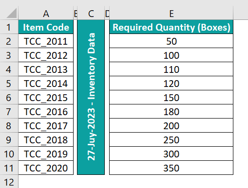
But the requirement is to randomly decide the quantities for the listed items instead of entering the values in ascending order.
Then, we can apply the concept of randomize a list of numbers in Excel using the Excel RAND function in a helper column.
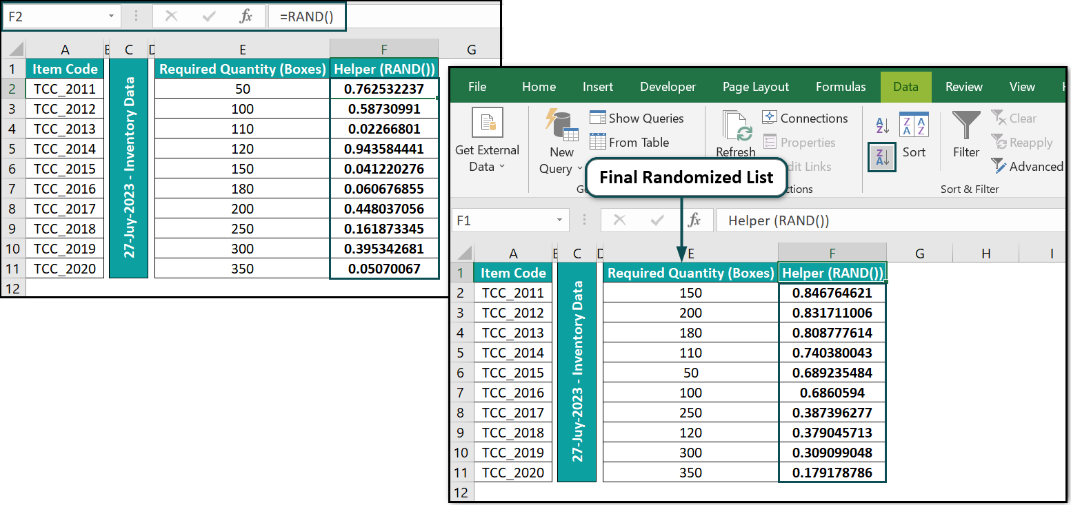
In the above randomize a list of numbers in Excel example, we add a new column F, titled Helper (RAND()), adjacent to column E containing the required quantities.
And then, we use the RAND() in cells F2:F11 to enter random numbers in the helper column against the column E values. Next, we select cells F2:F11, press Ctrl + C, and then Alt + E + S + V to copy and paste the column F data as values. We do so since the RAND() is volatile, and proceeding with the next steps will refresh the RAND() outputs in cells F2:F11, affecting the outcome.
And then, we select cells F2:F11 and choose the Sort Z to A option in the Data tab to sort the random numbers in descending order. And while sorting, we shall select the option to expand the sorting selection to column E values in the Sort Warning dialog box.
Thus, the above steps will randomize list in Excel column E, with the required quantities randomly assigned to the listed items.
Table of contents
Key Takeaways
- Randomize list in Excel is the method of changing the order of the values in a specific list randomly based on an adjacent column of sorted random numbers.
- Users can randomize a list to make unbiased decisions, such as grouping people into teams and deciding on a winner based on a random name picker.
- We can use the RAND and RANDBETWEEN inbuilt Excelfunctions to randomize lists in Excel.
- We can use an INDEX, SORTBY, SEQUENCE, and RANDARRAY functions-based formula to achieve a randomized list without duplicates.
How To Randomize List In Excel?
We can randomize list in Excel using the following steps:
- Add a helper column to the given dataset.
- Choose the first cell of the helper column and enter the RAND().
The RAND() syntax is:

While the function takes no arguments as input, it returns a uniformly distributed random real number, with 0 <= real number < 1. - Using the Excel fill handle, update random numbers in the required cells in the helper column.
- Select the cells in the helper column containing the RAND() return values. And press Ctrl + C to copy the cell values. Next, press Alt + E + S + V to paste the data as values.
- Select the helper column heading and choose the Data tab → select the Sort option to open the Sort window.
- The helper and adjacent columns will appear selected, and the Sort window will open.
Set the Sort by field as the helper column using the field’s drop-down list and choose the required order from the Order field drop-down list.
- Click OK to view the random numbers in the helper column sorted in the chosen order.
On the other hand, the adjacent columns will show the values in a random order based on the helper column values’ sort order.
Furthermore, we can use the Excel RANDBETWEEN formula instead of the RAND().
The RANDBETWEEN() syntax is as follows:

The function accepts two mandatory arguments, bottom and top. While the bottom is the smallest integer the function can return, the top is the largest integer it can return.
And it returns a random integer between the specified values, with the function return value changing every time we update, refresh, or open the worksheet.
Examples
Let us see a few examples to avoid the possibility of randomize list in Excel not working and hence achieve the desired outcome to meet our requirements.
#1 – Insert Random Numbers In The List By Using RAND Function
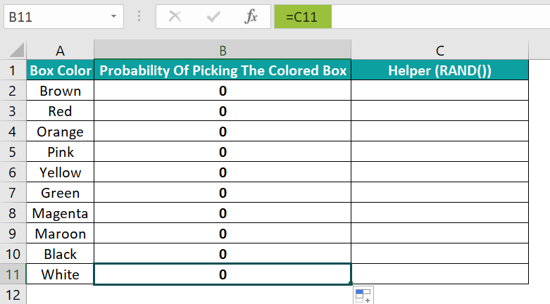
The table below shows a list of box colors.
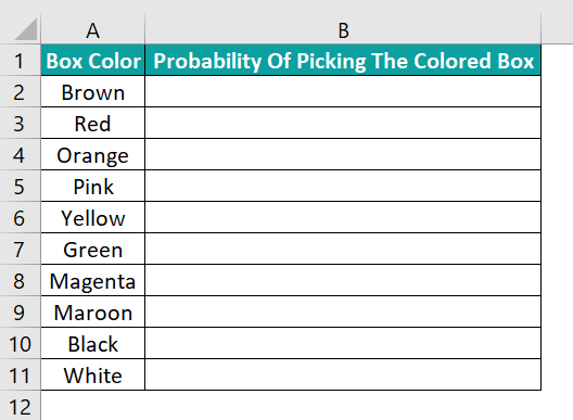
And the task is to determine the random probability of picking a specific color box and display the output in column B.
Then here is how to create and randomize list in Excel column B using the RAND().
- Step 1: Make column C a helper column.

- Step 2: Choose cell B2, enter the following formula, and press Enter.
=C2
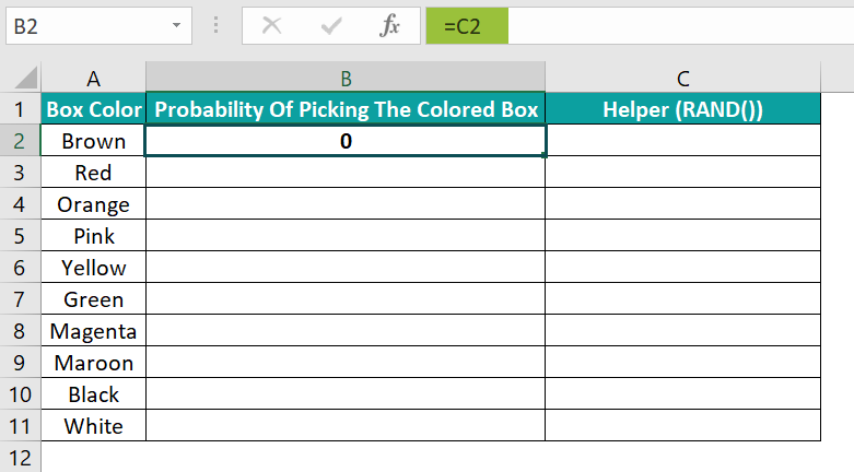
- Step 3: Update the formula in cells B3:B11 using the fill handle.
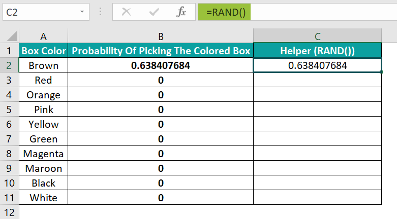
- Step 4: Choose cell C2 and enter the RAND().

- Step 5: Press Enter to view a random real number in the target cell C2.
- Step 6: Update the RAND() in the remaining cells C3:C11 to generate random numbers.
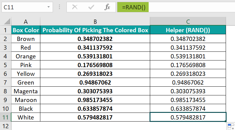
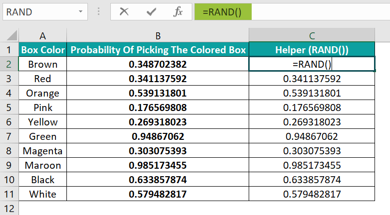
The random numbers get updated in column B automatically.
And, every time we refresh the formulas or edit the worksheet, the required random probability values get updated.

#2 – Pick A Lottery Winner With Randomize List In Excel
The following table contains a list of lottery ticket numbers.
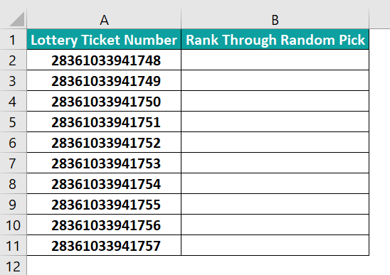
And the requirement is to determine the winning ticket number based on the rank through a random pick. The logic is to consider the person with the lottery ticket number picked first as the winner.
Then, we can create and randomize list in Excelcolumn B of ranks using the RAND().
- Step 1: Label column C as a helper column. And then, select cell C2, enter the RANDBETWEEN(), and press Enter.
=RANDBETWEEN(1,10)
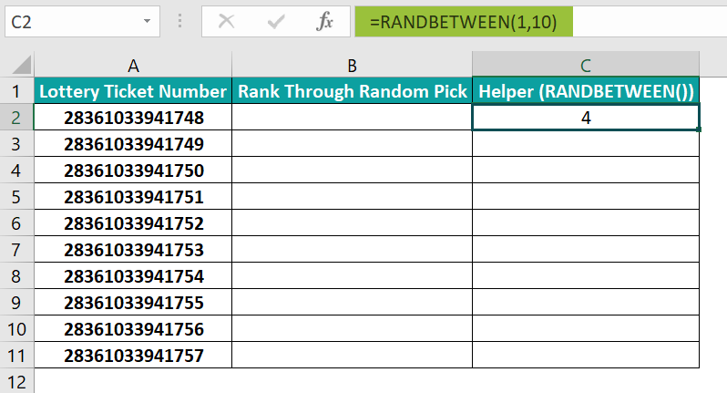
- Step 2: Using the fill handle, update the RANDBETWEEN() in cells C3:C11.
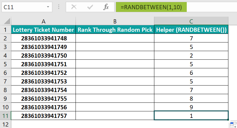
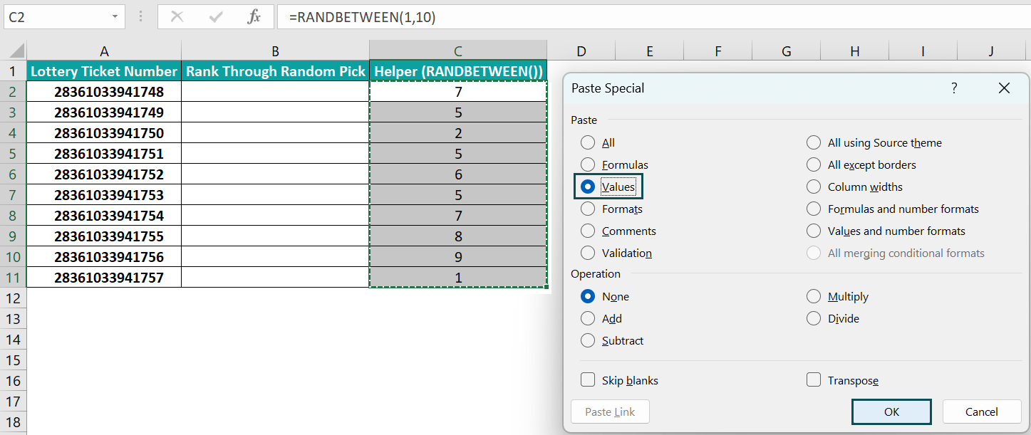
So, now column C contains repeated random numbers.
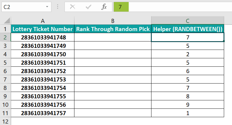
Next, as the RANDBETWEEN() output keeps changing each time we refresh or edit the worksheet, we shall copy and paste the obtained random numbers as values.
- Step 3: Select cells C2:C11 and press Ctrl + C to copy the values.
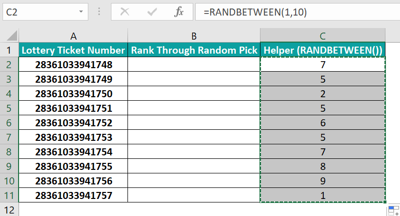
And press Alt + E + S + V to open the Excel Paste Special window and choose the Values option. And click OK to paste the cells’ data as values.
- Step 4: Choose cell B2, enter the following formula, and press Enter.
=RANK.EQ(C2,$C$2:$C$11)+COUNTIF($C$2:C2,C2)-1
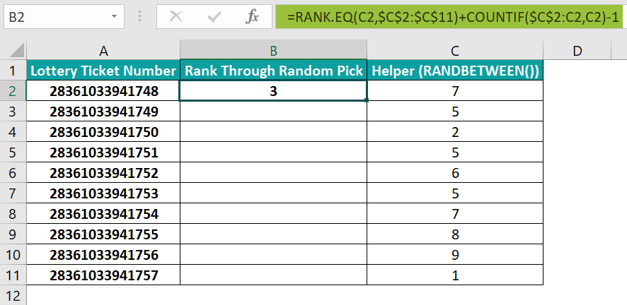
And then, using the fill handle update the formulas in cells B3:B11.
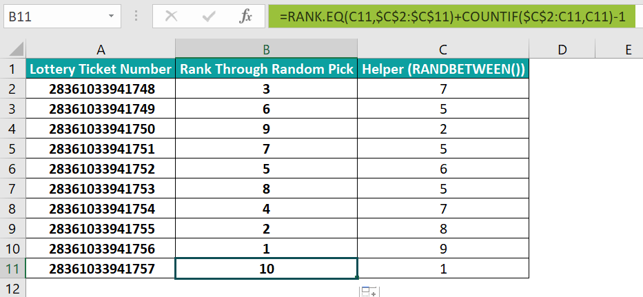
The Excel RANK function, RANK.EQ(), returns the rank of the number in the given list. And the size of the number is relative to the other numbers in the list.
Further, if more than one number has the same rank, the function returns the rank at the top.
And the Excel COUNTIF function counts the number of cells based on the specified criterion.
So, let us check the cell B11 formula to determine how the function works. First, the RANK.EQ() returns the rank of the value 1, 10. Next, the COUNTIF() returns the count of the total cells containing the value 1, 1. And hence, the formula evaluates as shown below:
=10+1-1
=10
Thus, the above formula in cells B2:B11 return unique values.
- Step 5: Click on a cell in the dataset and choose Data → Sort to open the Sort window.
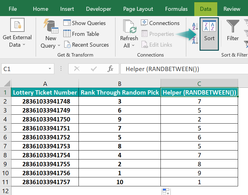
- Step 6: Click the Sort by field drop-down button to set the field as the helper column.

And then, click the Order field drop-down button to select the Largest to Smallest option.

Next, click OK in the Sort window.

Thus, the random values in the helper column are sorted in descending order.
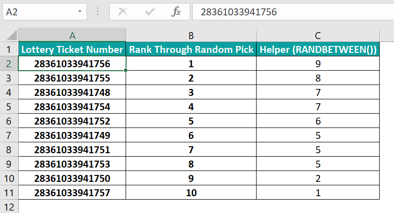
And the adjacent columns A and B values also get sorted automatically and randomly, based on the helper column values sorted in descending order.
Furthermore, we can consider column B as the randomized list. And hence, the lottery enthusiast possessing the lottery ticket number ranking number one can be declared the winner.
Thus, properly and practically using the RANDBETWEEN() syntax will ensure we avoid the scenarios of randomize list in Excel not working.
Benefits
The benefits of randomize list in Excel are as follows:
- It helps make unbiased decisions.
- It helps maintain data confidentiality.
- We can randomize the given list by changing the data order without manipulating it directly. And since we use a helper column of random numbers, the original data remains unmodified.
Important Things To Note
- The RAND and RANDBETWEEN functions are volatile. So, while they can slow down the program, their outputs get updated every time we refresh or edit the worksheet. Hence, it is best to copy and paste special function outputs when using them for randomize list in Excel.
- The RAND() will return unique real random numbers between 0 and 1 in the chosen cells. But the RANDBETWEEN() returns values between the specified numbers in the chosen cells. But the RANDBETWEEN function output may be repetitive.

Frequently Asked Questions (FAQs)
We can randomize a list in Excel into groups using the RAND(), RANK(), ROUNDUP(), and CHOOSE().
For example, the following table lists participants.
And the task is to divide them into four groups randomly.
Then, here is how to randomize a list in Excel into groups.
• Step 1: We shall use column B as the helper column. So, choose cell B2, enter the RAND(), and press Enter.
And using the fill handle, update the formula in the remaining cells B3:B13.
• Step 2: As the RAND() output keeps changing, we shall copy column B data and paste the data as values. And for that, select the range B2:B13 and press Ctrl + C.
And then, press Alt + E + S + V to open the Paste Special window and choose Values to paste the chosen cells’ data as values.
Next, click OK to complete the action.
• Step 3: Choose cell C2, enter the following formula, and press Enter.
=CHOOSE(ROUNDUP(RANK(B2,$B$2:$B$13)/3,0),”Team A”,”Team B”,”Team C”,”Team D”)
And then, using the fill handle, update the formula in cells C3:C13.
Thus, we will see the randomized list within the four groups (Teams A, B, C, and D).
Let us check the cell C13 formula to understand how it works.
First, the RANK() determines the rank of 0.718677438 based on the value size among the column B values, 5. Next, the RANK() output gets divided by 3, and we get a value of 1.66666666666667. And then, the ROUNDUP() rounds up the value to 2.
Finally, the CHOOSE() chooses the team name in the second position among the given team name options, Team B, as the last participant’s team.
The steps to randomize a list of names in Excel are as follows:
1) Label the column adjacent to the column containing names as Helper.
2) Select the helper column’s first cell, enter the RAND(), and press Enter.
3) Using the fill handle, update the RAND() in the required cells in the helper column.
4) Choose the cells in the helper column and press Ctrl + C to copy the value. And then, press Alt + E + S + V to open the Paste Special window and choose Values to paste the obtained random numbers as values in the helper column.
5) Click on a cell in the dataset and choose Data à Sort.
6) The Sort window opens. Set the Sort by field as the helper column and the Order field as Smallest to Largest or Largest to Smallest.
7) Click OK in the Sort window.
The list of names adjacent to the helper column gets sorted randomly. And hence we achieve the required randomized list of names.
We can randomize a list in Excel without duplicates using the following formula in the first cell of the column, where we must display the randomized list without duplicates:
=INDEX(SORTBY(SEQUENCE(Count_of_rows_to_return,1,Start_value_in_the_sequence,Step), RANDARRAY(Count_of_rows_to_return)),SEQUENCE(Total_random_numbers_to_display))
Download Template
This article must be helpful to understand the Randomize List In Excel, with its formula and examples. You can download the template here to use it instantly.
Recommended Articles
This has been a guide to What Is Randomize List In Excel. We explain how to randomize a list in Excel along with step by step examples. You can learn more from the following articles –


Leave a Reply