
What Are Ribbons In Excel 2019?
Ribbons in Excel 2019 are the sets of inbuilt commands grouped under different tabs based on their functionalities and featured at the top of the Excel work area. And the commands in the ribbon appear as icons and buttons.
Users can use the Excel ribbon to quickly find, understand, and apply the required commands to complete their tasks.
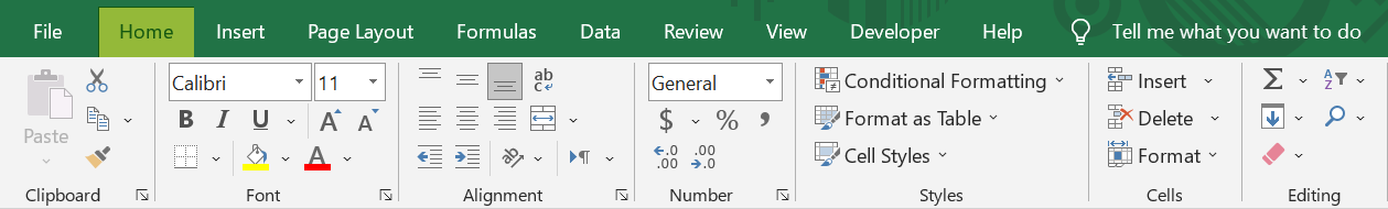
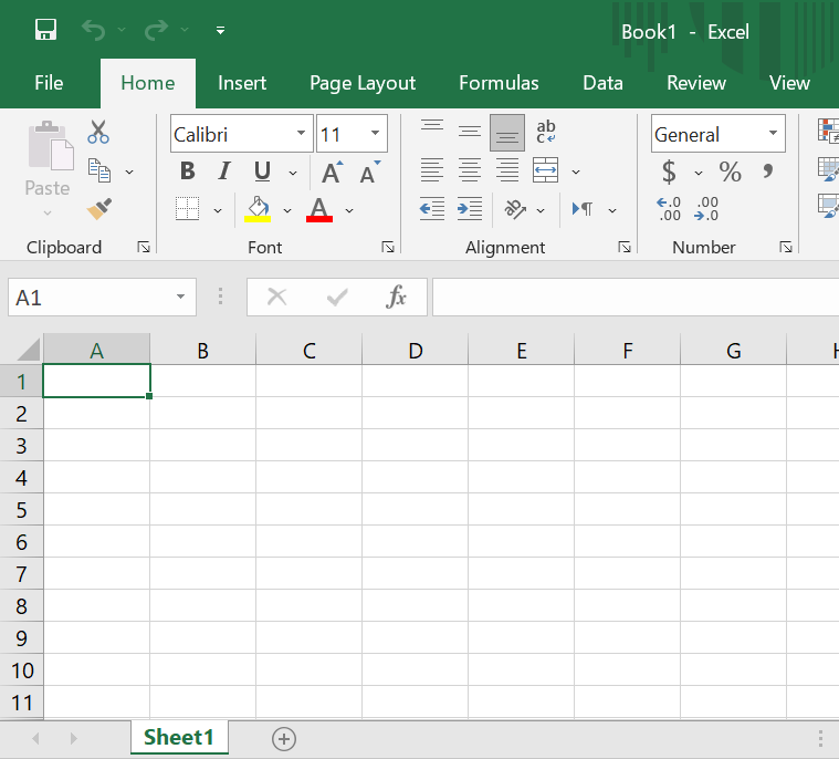
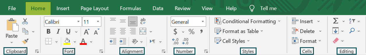
The image below shows the Excel ribbon with the Home tab open.
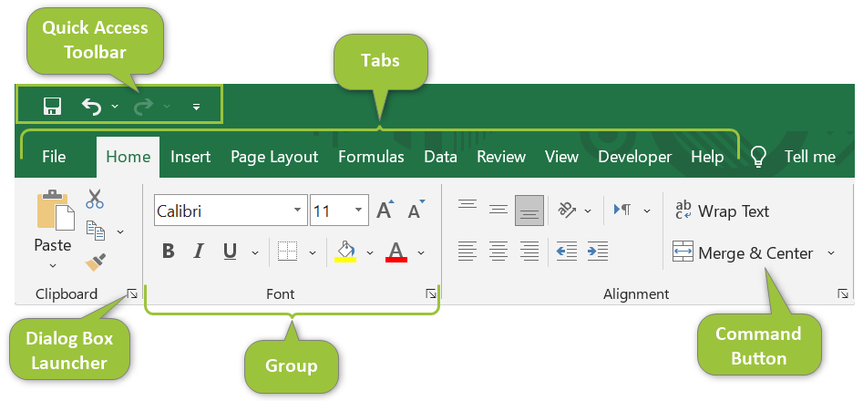
And a ribbon consists of the elements highlighted along with the Quick Access Toolbar in the following image.
Key Takeaways
- The ribbons in Excel 2019 are the primary interface, containing the frequently used commands and features in the form of icons and buttons.
- The tabs in Excel 2019 are the categories in which the Excel commands and features are grouped based on their functionalities. Excel, by default, shows nine tabs in a worksheet. And additionally, there are two tabs that users can unhide and use according to their task demands.
- The Quick Access Toolbar in Excel 2019 shows a set of command shortcuts independent of the tab open in the ribbon.
How To Open The Excel 2019 Software?
The steps to open the Excel 2019 software in Windows are as follows:
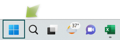
- First, press the Windows icon on the left-bottom corner of the Windows taskbar to open the Windows Start menu.
[Alternatively, we can press the Windows key on the keyboard.]

- Next, scroll down the Program files list to the letter E and then, click on Excel to open Excel 2019 from the Start menu.

Alternatively, type Excel in the search field next to the Windows icon on the left-bottom corner of the Windows taskbar. And then, click on Excel from the list of matching programs.
Then, click on Excel. It will open the Excel 2019 software window.


How To Open A Blank Workbook In Excel 2019?
The steps to open a blank workbook in Excel 2019 are as follows:
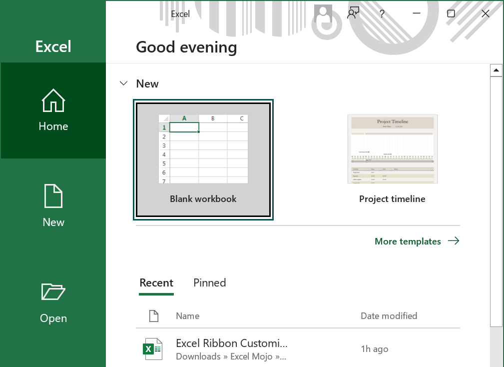
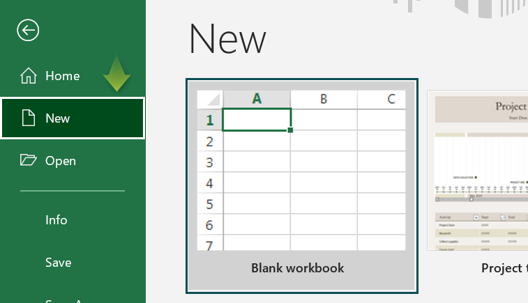
- Step 1: To begin with, click the Blank workbook option, once the Excel 2019 software opens, as highlighted in the image below.
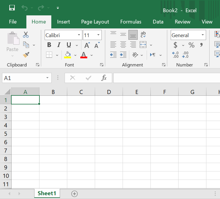
The above action will open a blank workbook, as shown below:
On the other hand, if we have a workbook open and wish to open a new blank workbook, then the steps are as follows:
- Step 1: First, click File → New.

Next, click on the Blank workbook option as shown below:
The above step will open a new empty workbook.
How To Collapse (Minimize) Ribbons?
Ideally, the preference is to show ribbons in Excel, which helps quickly access inbuilt commands and features.
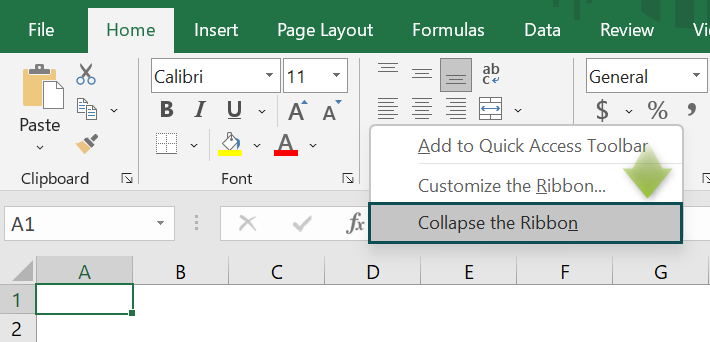
However, in some scenarios, we may require to minimize or collapse it. So, here is how to collapse the Excel ribbon and display it as shown below:
- Step 1: To begin with, right-click on the ribbon to open the context menu. Then, click the option Collapse the Ribbon to minimize the ribbon.
How To Customize Ribbons?
Though we prefer to show ribbons in Excel, which we use frequently, it is also possible to customize ribbons.
We shall see how to add tabs in Excel ribbon as the ribbon customization.
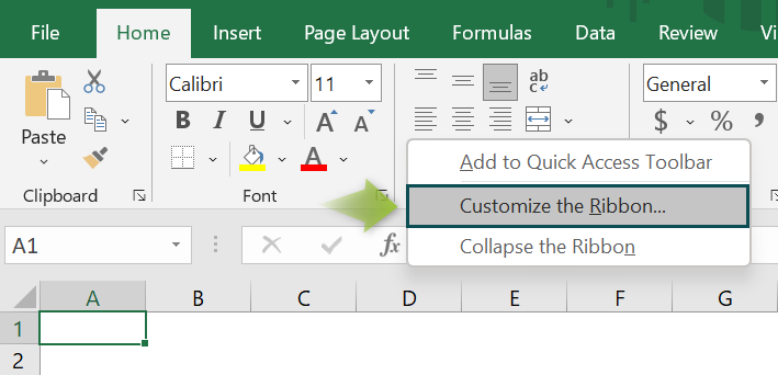
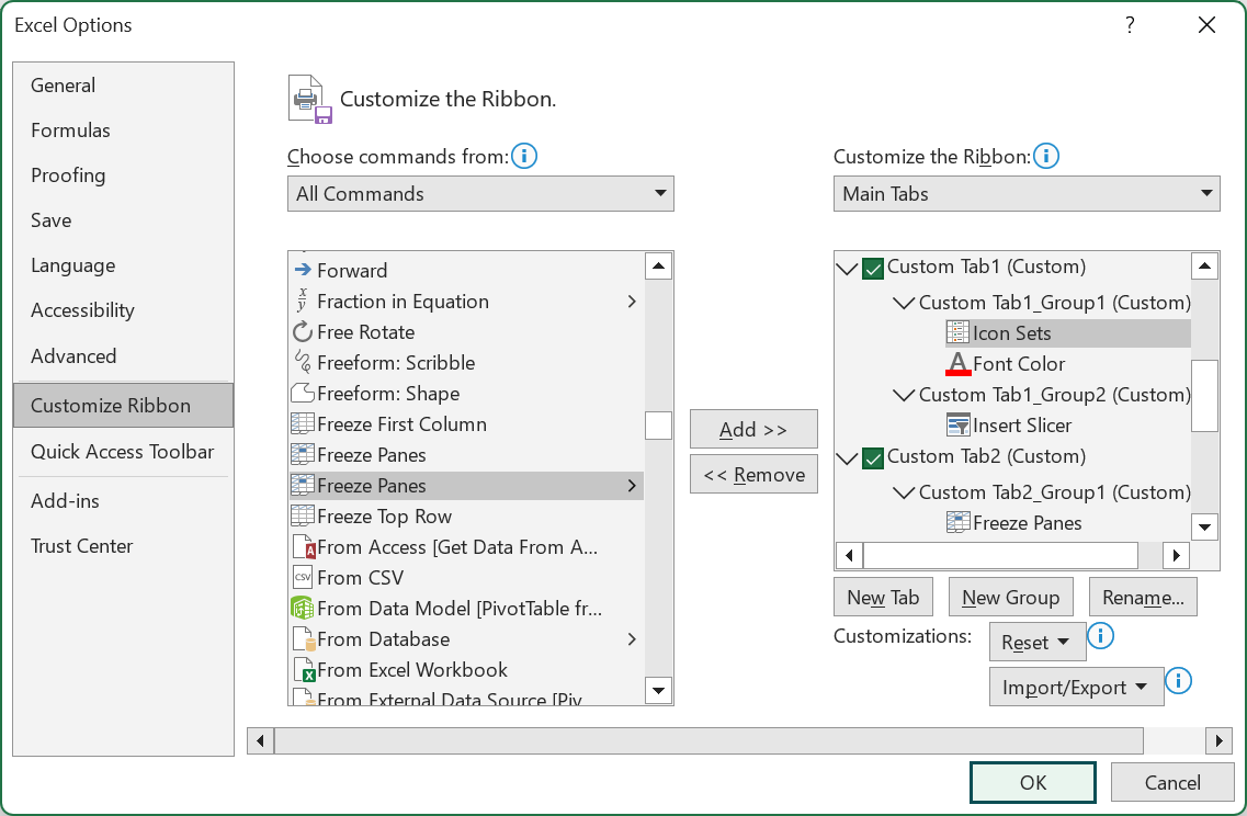
- Step 1: First, right-click the ribbon in the active worksheet. Next, pick Customize the Ribbon from the context menu to open the Customize Ribbon tab in the Excel Options window.
[Alternatively, click File → Options to open the Excel Options window.

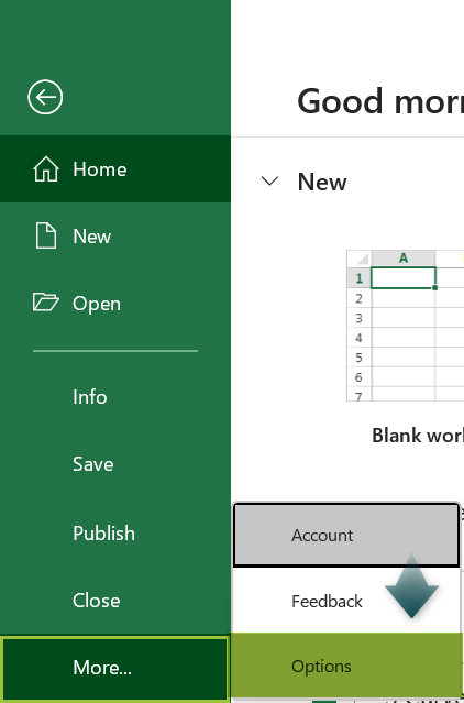
And then, open the Customize Ribbon tab in the Excel Options window.]
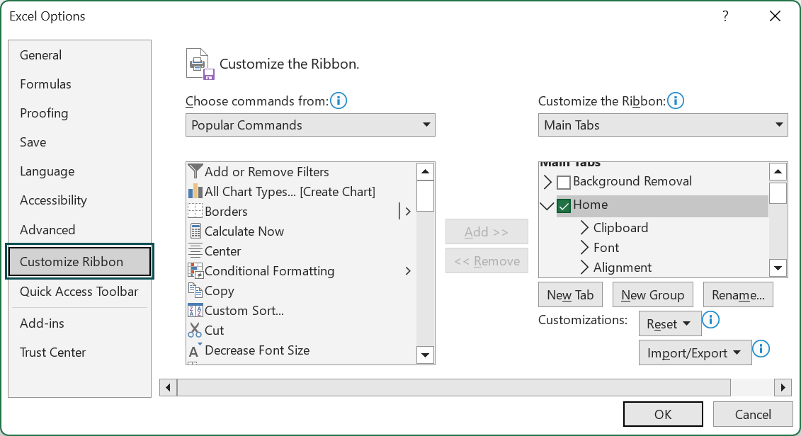
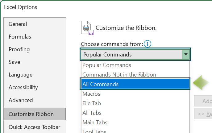
- Step 2: Next, using the drop-down button, set the Choose commands from field as All Commands.
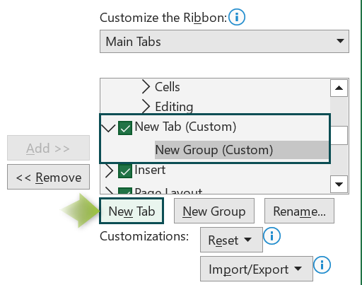
- Step 3: Then, press New Tab to insert a new tab in the Main Tabs list.
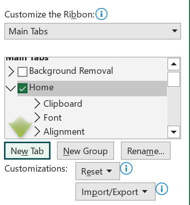
Next, press New Tab again to create another new tab in the Main Tabs list.
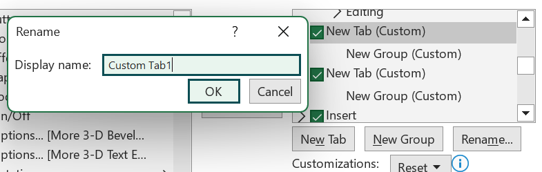
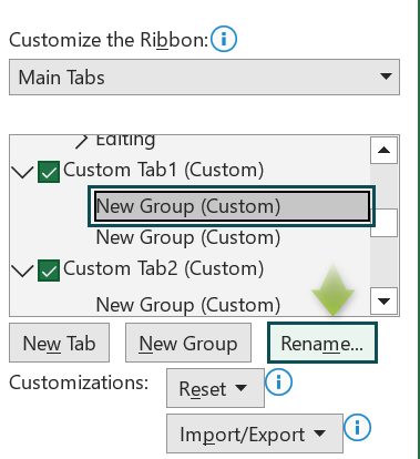
- Step 4: Now, click on the first new tab and press Rename.
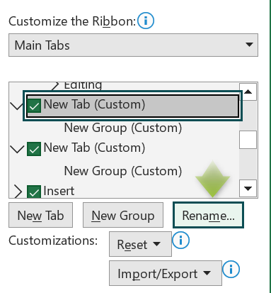
Next, the Rename window will open. Here, we need to enter the new tab display name. Then, click OK.
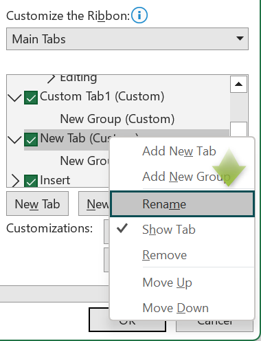
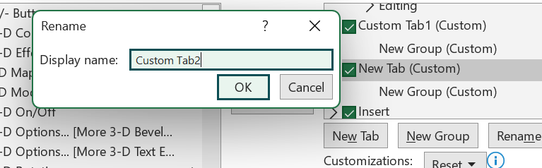
Likewise, update the second new tab’s name. Also, we can right-click on the entity we wish to rename and click Rename in the context menu to open the Rename window and update the display name.
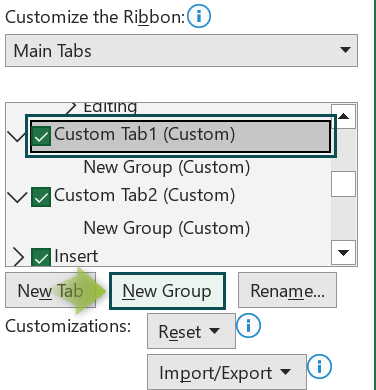
- Step 5: Next, click the first custom tab and then, press New Group to add a new group to the tab.
Now, click the first group in the first custom tab and then, press Rename to rename the group.
The Rename window opens, where we must enter the required group name and click OK.
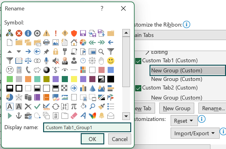
Likewise, update the names of the remaining groups in the new tabs.
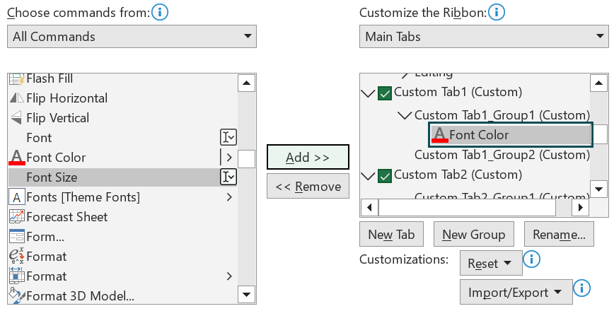
- Step 6: Next, select the first group in the first custom tab, pick the command from the All Commands list required in the chosen group, and then, press Add.
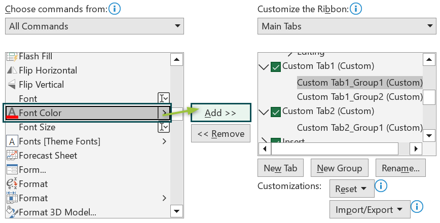
Similarly, insert the commands required in the specific groups in the custom tabs using Add, one at a time. And we can update the command names in the custom tabs using the Rename option.
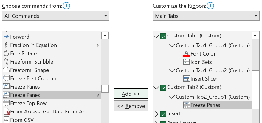
- Step 7: Now, we can reorder the commands within the group. For example, click the Insert Icons command and then, press the Move Up button.
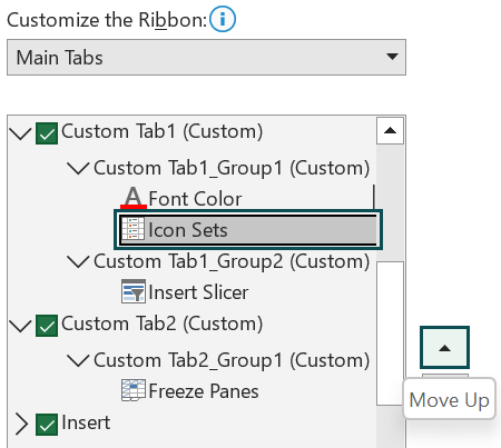
Likewise, we can reorder the groups within the custom tabs and rearrange the custom tabs’ order.
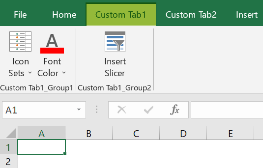
- Step 8: Next, click OK to view the two new custom tabs in the Excel ribbon.
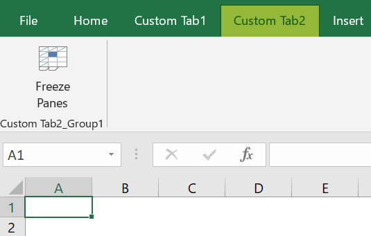
We can also remove commands, groups, and tabs by selecting the specific element and clicking the Remove option.
The above customization steps are possible when we create a new tab in the ribbon. However, we cannot perform a few actions with the inbuilt commands in the standard ribbon tabs. For example, we cannot rename or reorder them, though renaming and reordering the groups in the standard tabs are possible.
What Is Quick Access Toolbar?
The Quick Access Toolbar is available at the top-left corner of the Excel window. It is a set of shortcuts to frequently used Excel commands, options, and features. And the toolbar is independent of the ribbon tab currently open in the worksheet.
Further, the toolbar is customizable. While we can add new command to Quick Access Toolbar in Excel, removing the commands from the toolbar is also possible. Also, we can place the toolbar above or below the ribbon in the worksheet.
How To Customize Quick Access Toolbar?
We shall see how to add new command to Quick Access Toolbar in Excel as the customization.
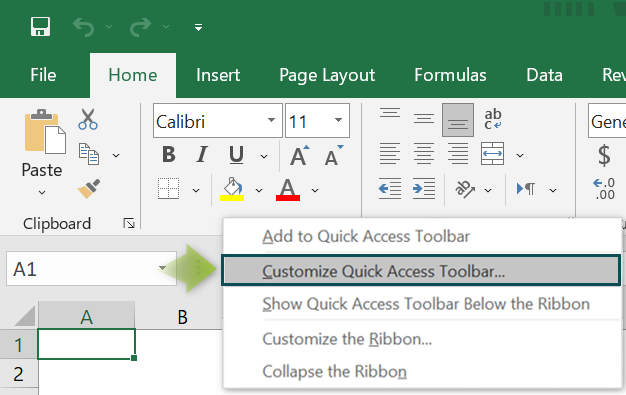
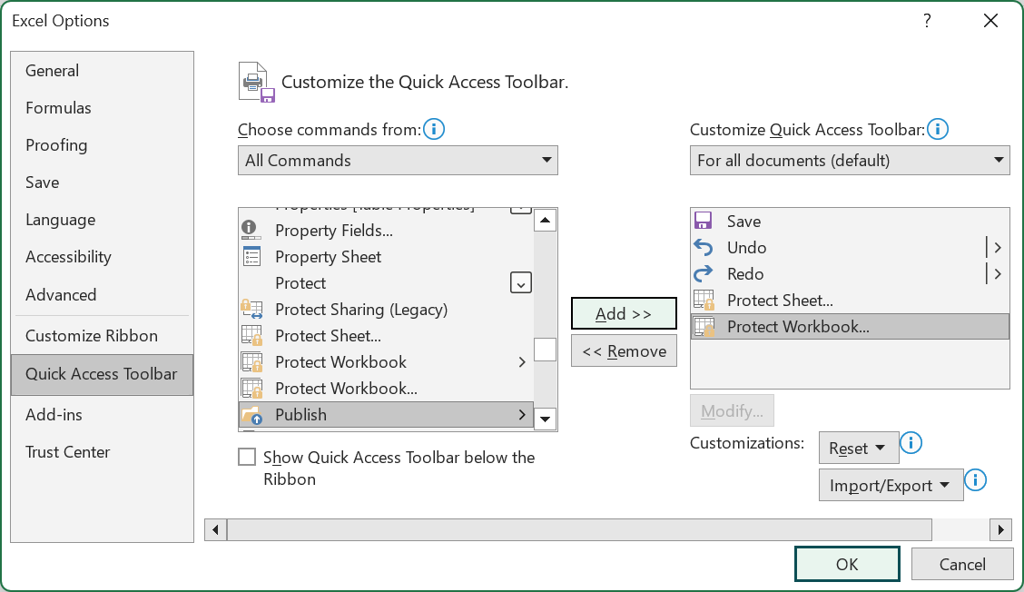
- Step 1: To start with, right-click on the ribbon in the current worksheet and pick Customize Quick Access Toolbar from the context menu. Now, the action will open the Quick Access Toolbar tab in the Excel Options window.
[Alternatively, click File → Options to open the Excel Options window.
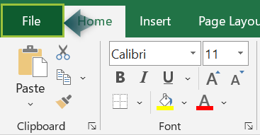

And then click the Quick Access Toolbar tab in the Excel Options window.]

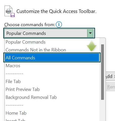
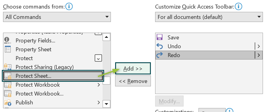
- Step 2: Next, the tab will show the existing commands in the Quick Access Toolbar under the Customize Quick Access Toolbar field. And as we require to add new commands in the toolbar, pick All Commands in the Choose commands from field.
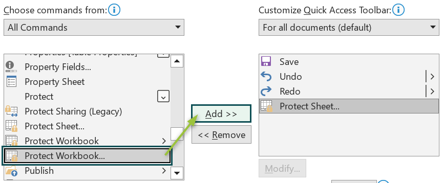
- Step 3: Then, we will add the Protect Sheet and Protect Workbook commands in the toolbar. And for that, we must pick one command and click Add to add the commands one at a time to the toolbar.
On the other hand, we can use the Remove option to delete commands from the toolbar.
- Step 4: Next, click OK.
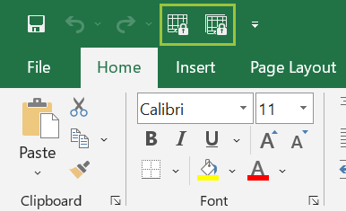
Clicking OK will close the Excel Options window, and we will see the chosen commands added in the Quick Access Toolbar in the active workbook.
What Are The Tabs?
The Excel ribbon organizes the closely-related inbuilt features and commands into tabs above the work area. And while Excel 2019 shows nine tabs by default, one can add tabs in Excel according to their task demands.
When we open an Excel sheet, we typically see the tabs shown below.

But, once we unhide all the tabs using the options in the Customize Ribbon tab in the Excel Options window, we will find the tabs shown in the image below when we view tabs in Excel.

Now, let us see the important ones in this section.
#1 – Home Tab
When we view tabs in Excel worksheet, we will see the Home tab open by default.
- Clipboard
The Cut, Copy, and Paste commands help cut, copy as is and as a picture, paste as is, and paste special. Thus, we can use these options to cut or copy data from the source location to delete and paste or to retain the data in the source location and paste data in the target cells.
Similarly, we can paste the copied data with formulas or in the desired format using the Paste Special option.
Next, the group includes the Format Painter option, which applies the source cell format to the target cell.
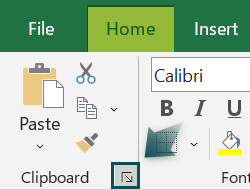
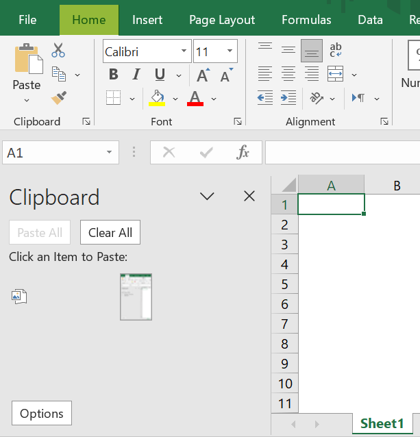
Further, clicking the Clipboard dialog box launcher will open the Clipboard pane.
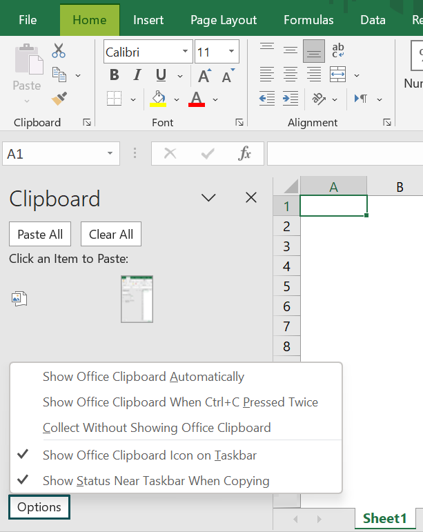
Meanwhile, we can click the images listed in the pane to paste them into the worksheet. Also, we can use Options to manage the Clipboard settings.
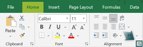
- Font
The Font group contains options for applying the desired fonts in the Excel cells and changing the font size. It also includes options to make the cell content bold, italic, and underline the chosen cell data.
Further, it includes options to set the desired cell borders and cell and font colors.
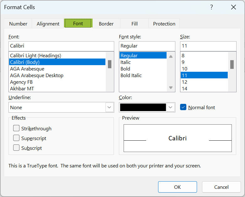
And clicking the Font dialog box launcher opens the Font tab in the Format Cells window.
While one can also set the above mentioned settings from this tab, the tab shows an additional command, Effects. We can use it to enter data in a cell with the chosen effect.

- Alignment
The Alignment group includes the cell data horizontal and vertical alignment options, Top, Middle, Bottom, Left, Center, and Right. And we can set the required cell data orientation and indent settings.
Furthermore, it contains the Wrap Text option in excel, which enables one to show the entire extra-long data in multiple lines in a cell. And we can merge and unmerge Excel cells using the Merge & Center in excel option.
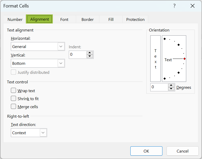
Meanwhile, after we click the Alignment dialog box launcher, it opens the Alignment tab in the Format Cells window.
Also, the tab shows a few more features to help us control cell text better.
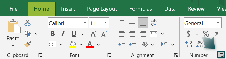
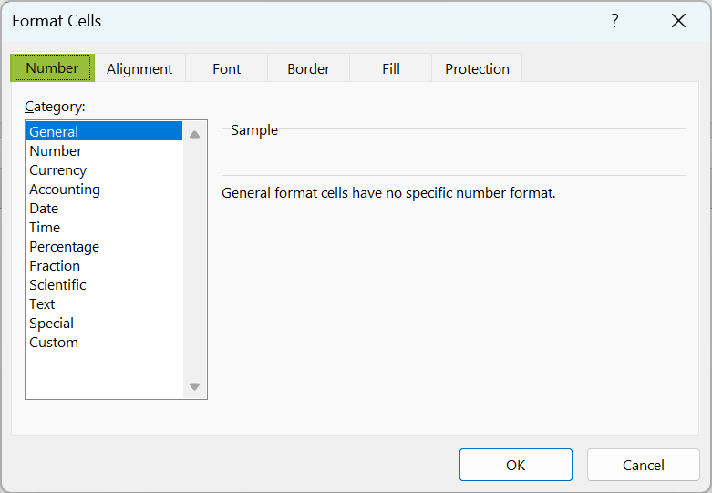
- Number
The Number group lets one change the number format, currency settings, percent, and comma styles and increase and decrease decimal places in Excel cells.
And clicking the Number dialog box launcher opens the Number tab in the Format Cells window.
Similarly, users can set customized number formats in Excel cells from this Number tab.
- Styles
The Styles group includes three features.
The Conditional Formatting option identifies patterns in the chosen data and highlights values using colors and icons.
On the other hand, the Format as Table option converts the specified data range into a table with a chosen style.
Likewise, the Cell Styles option helps highlight critical data in a data range.
- Cells
The Cells group includes three commands.
The Insert and Delete commands help add and delete cells, rows, columns, and worksheets in workbooks.
Also, the Format option helps adjust cell height and width and hide and protect cells.
- Editing
The Editing group contains five commands.
While AutoSum automatically adds calculations to a selected data range, Fill allows one to continue patterns in neighboring cells in the chosen direction.
And Clear removes everything in chosen cells. It also helps remove specific aspects such as formats, content, comments, and hyperlinks in the selected cells.
Furthermore, the Sort & Filter feature helps organize and sort data in the desired order and filter data. Thus, the command makes data analysis more straightforward.
And the Find & Select feature helps find data in the file. And it offers advanced search options to narrow the searches and even replace data.
#2 – Insert Tab

- Tables
The Tables group contains three features, PivotTable, Recommended PivotTables, and Table.
The PivotTable arranges and summarizes complex data in pivot tables. On the other hand, the Recommended PivotTables allows Excel to suggest customized pivot tables that best suit the specified data.
Also, the Table option creates an Excel table with the given data, making data sorting, filtering, and formatting more straightforward.
- Illustrations
The Illustrations group commands help insert pictures from the computer and online, shapes and icons, 3D models, and graphics in the Excel worksheet. And the group also includes an option to take screenshots.
- Add-ins
The Get Add-ins and My Add-ins commands help browse and manage add-ins in worksheets.
We can use the third command to visualize data using Visio diagrams in Excel. And the Bing Maps app helps plot locations and visualize Excel data using Bing Maps.
And the last command in this group converts data into vivid pictures, which makes data interpretation more straightforward.
- Charts
The Recommended Charts and the eight chart categories enable users to insert the desired chart to represent their data graphically for visual analysis.
On the other hand, the Maps option inserts Map charts to compare data and show categories across geographical regions.
Furthermore, the Pivot Chart excel feature graphically summarizes complex data.
- Tours
The Tours group contains only one feature, 3D Map. It helps visualize geographic data on a 3D map over time.
- Sparklines
The Sparklines excel group includes three Sparklines commands. The commands help insert mini charts in cells, each representing a row of data in the chosen data range.
While the Line option inserts Line sparklines, the Column option inserts Column sparklines. And the Win/Loss option creates a Win/Loss sparkline.
- Filters
The Slicer excel feature in the Filters group helps filter tables, pivot tables, pivot charts, and cube functions.
On the other hand, the Timeline option assists in quickly selecting periods for filtering tables, pivot tables, pivot charts, and cube functions.
- Links
The Links group contains one command, Link, which helps insert links in cells to other locations in the Excel files and documents, files on the computer, and webpages.
- Text
The Text group contains the Text command to insert text boxes, headers & footers, WordArt, signature lines, and objects.
- Symbols
The Equation feature in the Symbols group inserts mathematical equations in worksheets. On the other hand, the Symbol option helps add symbols to the worksheets, which are not available on the keyboard.
#3 – Page Layout Tab
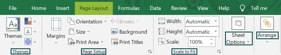
- Themes
The Themes group includes four features, Themes, Colors, Fonts, and Effects.
While Themes helps set the desired theme for the Excel document, the Colors option changes the color palette used in the workbook. And the Fonts option is useful for picking the desired font set to show data in a workbook.
Further, we can use the Effects option to change the appearance of objects in the workbook quickly.
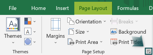
- Page Setup
The commands in the Excel Page Setup group enable users to update the page settings when printing Excel data to obtain the printed data in the desired format.
While the Margins option adjusts and customizes the margin, the Orientation command changes the page orientation. And the Size command helps pick a page size.
On the other hand, the Print Area command is useful for selecting an area in the sheet we wish to print.
Furthermore, the Breaks option adds a break where we wish the next page should start when we print the worksheet content. And the Background command inserts the picture of our choice in the Excel content background.
Likewise, the Print Titles option allows one to choose the rows and columns required to appear on all the printed pages.
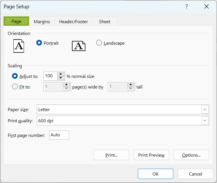
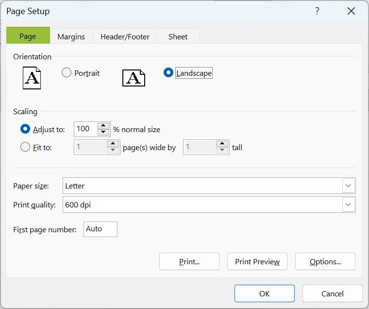
Further, clicking the Page Setup dialog box launcher will open the Page Setup window. And we can apply additional page setup setting from the Page tab in the Page Setup window.
- Scale to Fit
The Scale to Fit group includes three commands.
The Width and Height options reduce the printout width and height, respectively, to ensure it fits within the desired number of pages.
And the Scale command is useful to stretch or shrink the printout to a percentage of its original size.
And clicking the Scale to Fit dialog box launcher will open the Page Setup window.
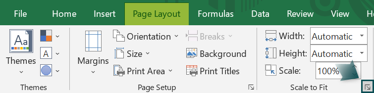
We can apply the additional scale to fit settings from the Page Setup window.
- Sheet Options
The Sheet Options group includes two commands, Gridlines, and Headings.
The Gridlines command allows users to view the gridlines in worksheets and printouts. And the Headlines option lets one view the row and column headings in worksheets and printouts.
Moreover, clicking the Sheet Options dialog box launcher opens the Sheet tab in the Page Setup window.
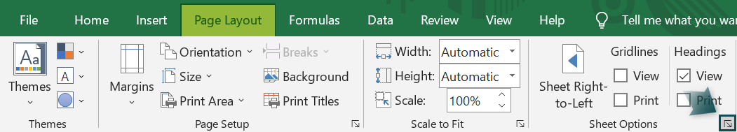
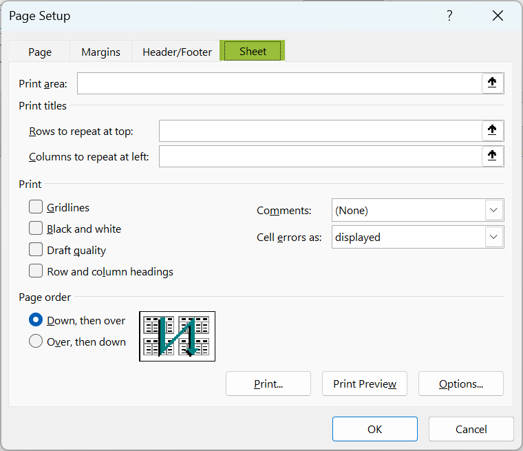
We can use additional sheet setup options to achieve the Excel data printouts in the desired format.
- Arrange
The Bring Forward command in the Arrange group brings the chosen object one step forward or in front of all other objects in the worksheet.
And the Send Backward option sends the chosen object one step back or behind all other objects in the worksheet.
Furthermore, the Selection Pane option helps view the list of objects in the worksheets. And the Align command changes the position of the objects on the Excel page.
The Group feature joins objects to manage them as a single object. And the Rotate command rotates the chosen object.
#4 – Formulas Tab
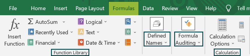
- Function Library
The Function Library group includes different categories of Excel inbuilt functions such as Financial, Logical, Text, Data & Time, Lookup & Reference, and Math & Trig.
On the other hand, it includes the Insert Function to select the required function from the Insert Function window. The group also has the More Functions option to access additional and Compatibility Excel functions.
Moreover, the AutoSum option has the same functionality as explained in the Home tab section. And the Recently Used option helps apply the functions we recently used.
- Defined Names
The Name Manager in excel is useful for creating, editing, deleting, and finding all the names in the workbook.
On the other hand, the Define Name option defines and applies names. And the Use in Formula command enables one to choose a name used in the workbook and use it in the specific formula.
Further, the Create from Selection option generates names from the chosen cells.
- Formula Auditing
Formula auditing excel features like Trace Precedents and Trace Dependents commands help manage the trace precedents and dependents. Similarly, the Remove Arrows option deletes the arrows the trace precedents and dependents draw.
Furthermore, the Show Formulas command displays the formulas instead of the values in the chosen cells. And clicking the Error Checking option will help check and trace the errors in the specific formulas.
And the Evaluate Formula feature enables one to check the step-by-step calculations when using a formula in a cell, which helps debug in case of incorrect results.
Additionally, the group includes an option, Watch Window. Also, it helps create a list of cells whose values we must monitor while working across other parts of the Excel sheet.
- Calculation
The Calculation Options feature in the Calculation group enables one to decide whether Excel should calculate manually or automatically.
And the Calculate Now and Calculate Sheet commands in the group are to calculate in the entire workbook and the active worksheet.
#5 – Data Tab
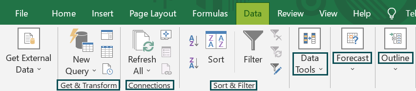
- Get & Transform Data
The Get Data feature enables one to explore, connect, and combine data from multiple sources to shape and refine to match the requirements.
And while the From Text/CSV option imports data from CSV files, the From Web command imports data from a webpage. On the other hand, the From Table/Range option creates a query linked to the chosen Excel table.
Moreover, the Recent Sources command helps manage and connect to the recent data sources. And the Existing Connections option assists in importing data from common sources.
- Queries & Connections
The Refresh All feature allows one to obtain the latest data by refreshing all the sources in the workbook. On the other hand, the option Queries & Connections helps view and manage the queries and connections in the workbook.
On the other hand, the Properties command helps users to analyze how the data range linked to a data source will update. And the Edit Links command helps view all the files the spreadsheet is linked externally and manage the external links.
- Sort & Filter
There are two commands in the Sort & Filter group, which help sort in ascending and descending orders. Meanwhile, the Sort function enables one to find the required values by sorting the data and the Filter command turns on the filter in the chosen cells.
Further, the Clear command clears the applied filters and sort state in the chosen cell range. And the Reapply command reapplies the applied filters and sort state in the chosen cell range.
On the other hand, the Advanced feature enables us to filter data using complex criteria.
- Data Tools
The Text to Column in Excel allows users to split a single data column into multiple columns. And Flash Fill automatically updates values in chosen cells.
Further, the Remove Duplicates command removes duplicate rows in a sheet.
The Data Validation feature helps pick from a list of rules to restrict the data types to enter into chosen cells.
Furthermore, the Consolidate command consolidates data from different cell ranges and displays the data in a single data range. And the Relationships command helps build or edit relations between tables to display the related data from the tables.
And the Manage Data Model feature is associated with the Power Pivot Window functionality to add and edit data.
- Forecast
The What-If Analysis feature allows users to try different values in the specified formulas in the worksheet using the Scenario Manager, Goal Seek, and Data Table options.
On the other hand, the Forecast Sheet command helps create a new spreadsheet to predict trends.
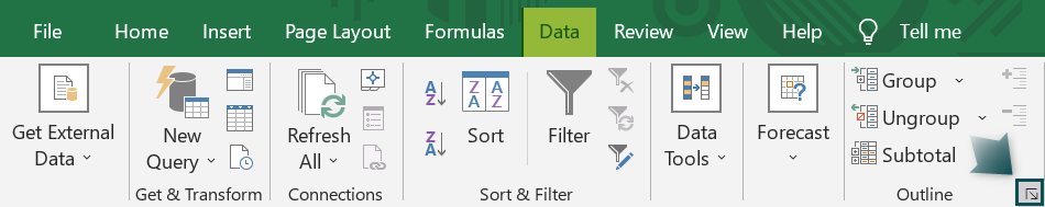
- Outline
The commands, Group and Ungroup, group ranges of cells and ungroup the cell ranges previously grouped. On the other hand, the Subtotal option evaluates rows of data using totals and subtotals.
Furthermore, the group includes two other commands, Show Detail and Hide Details to expand a collapsed cell group and collapse a group of cells.
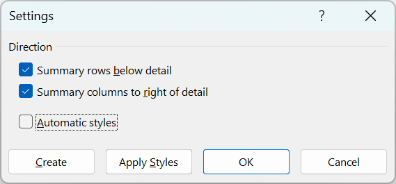
And clicking the Outline dialog box launcher opens the Settings window, where we can set the summary directions and styles.
#6 – Review Tab
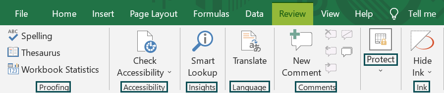
- Proofing
The Proofing group includes two features, Spelling,and Thesaurus.
While Spelling performs a spell check, the Thesaurus helps find synonyms.
- Accessibility
The group contains one command, Check Accessibility, to verify the Excel file follows the accessibility best practices.
- Insights
The Smart Lookup option in the Insights group enables one to understand the chosen text by looking up descriptions, images, and other sources online.
- Language
The Translate command in the Language group translates the chosen text into the desired language.
- Comments
The New Comment command in the Comments group inserts a comment in the chosen cell. And the Delete, Previous, and Next commands remove and jump to previous and next comments.
Furthermore, the group includes two more functions, Show/Hide Comment and Show All Comments. These options help one to display or hide comments in the chosen cells and display all the comments in the spreadsheet.
- Protect
The Protect Sheet and Protect Workbook commands protect the worksheet and workbook from unnecessary changes made by unauthorized parties.
On the other hand, the Allow Edit Ranges option helps password-protect data ranges.
And the Unshare Workbook feature helps to unshare an Excel file.
- Ink
The Start Inking command enables one to add a freehand pen and highlighter strokes in an Excel file. And the Hide Ink option helps hide the ink we added to our document.
#7 – View Tab

- Workbook Views
When we click the Normal option, we can view the Excel file in the normal view. On the other hand, the Page Break in excel option helps to see where the page breaks will appear when printing the Excel document.
Furthermore, the Page Layout function allows one to check how the printed Excel document will appear. And the Custom Views option enables us to save the print settings to apply in the future.
- Show
The Show group includes four options.
While the Ruler shows the rulers next to the worksheet, the Gridlines show the lines between the rows and columns in the worksheet.
Furthermore, the Formula Bar shows the Formula Bar above the work area, and the Headings option shows the row and column headings in the worksheet.
- Zoom
The Zoom command enables us to zoom the worksheet to the extent we require. And the next command zooms the worksheet to 100%.
On the other hand, the Zoom to Selection option zooms the chosen data range to fill the entire window.
- Window
The New Window command opens a second window for the current Excel file to work in both documents simultaneously. And the Arrange All option stacks all the windows to view them in one go.
Furthermore, the Freeze Panes in Excel enables one to select and freeze a cell range to keep them visible while scrolling through the rest of the worksheet.
The Split command divides the window into multiple panes, which we can scroll individually. On the other hand, the Hide option hides the active window, and the Unhide command unhides the hidden windows.
Moreover, the group includes four more commands.
The View Side by Side command helps view different workbooks adjacent to each other. And the Synchronous Scrolling command scrolls two documents simultaneously.
On the other hand, the Reset Window Position option lets us place the files side by side we wish to compare. Simialrly, the Switch Windows option helps to switch to another Excel window quickly.
- Macros
The Macros group contains one feature, Macros in Excel, which helps view the macros used in the Excel sheet.
Frequently Asked Questions (FAQs)
Ribbon in Excel may not work because of the following reasons:
• We opened the Excel file in the protected view.
• Our file is in Reduced Functionality Mode.
• We are trying to access an entirely collapsed ribbon in your Excel file.
We can unhide tabs in Excel using the Customize the Ribbon option. Let us see the steps with an example.
Suppose Excel shows the standard nine tabs.
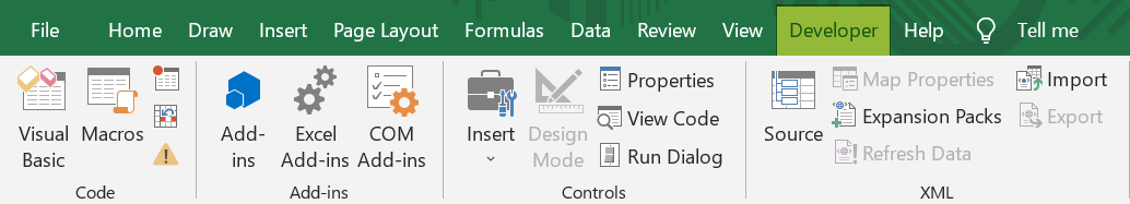
And the requirement is to unhide the Draw and Developer tabs. Then, the steps are as follows:
• Step 1: To begin with, right-click the ribbon and pick Customize the Ribbon option from the context menu.
Next, the Customize Ribbon tab in the Excel Options window pops up.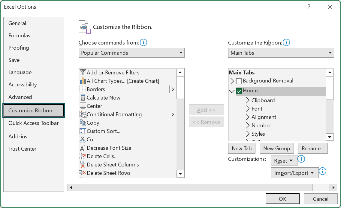
• Step 2: Now, check the Draw and Developer tabs’ boxes under the Main Tabs list. Then, click OK.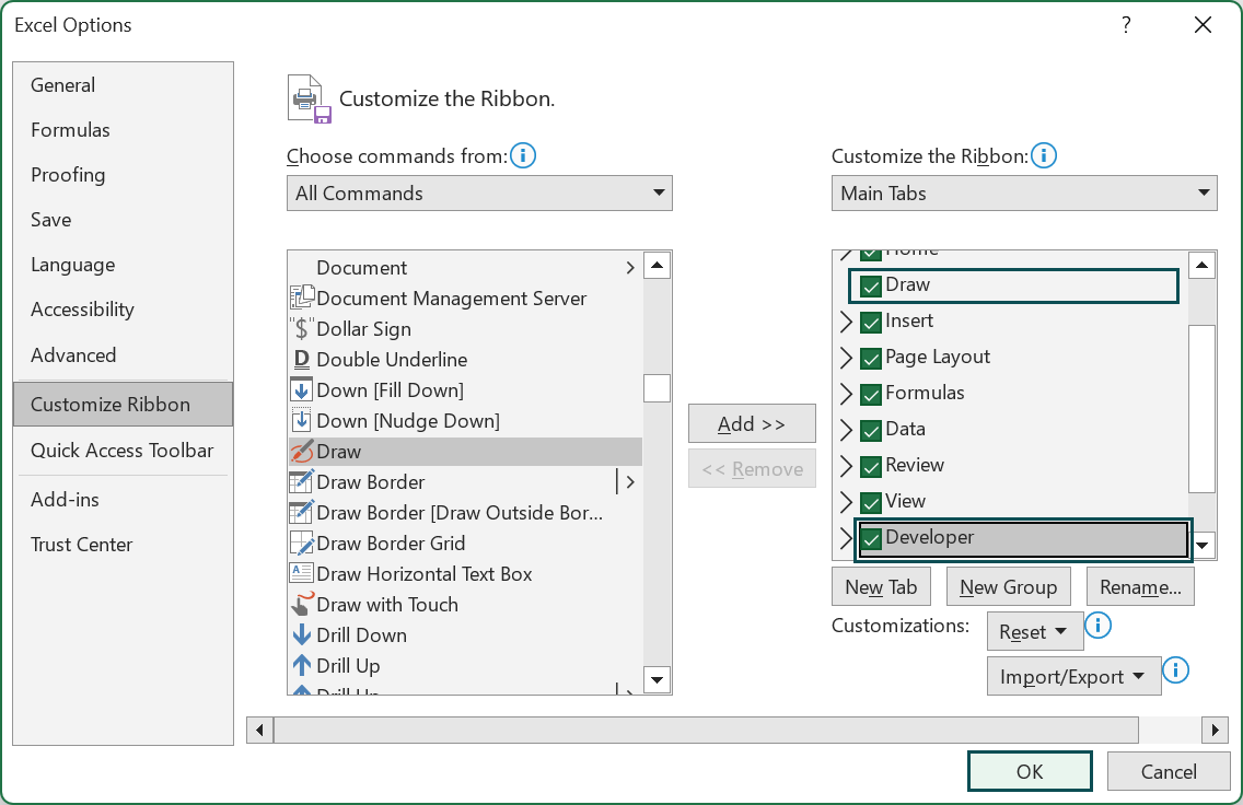
After we click OK, it will unhide the two chosen tabs, and they will appear in the Excel 2019 ribbon.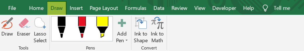
The purpose of Quick Access Toolbar in Excel is that it enables one to display and apply a set of Excel commands’ shortcuts independent of the tab currently open in the ribbon.
Further, the toolbar is customizable, and we can place it above or below the ribbon.